How to collapse all pivot table fields in Excel

A pivot table is a tool in Excel that allows you to summarize and organize large amounts of data. It allows you to rotate rows and columns to see different summaries of the data, and to create a summary table that can be easily sorted, filtered, and analyzed. Pivot tables can be used to quickly find patterns and trends in your data, and to make it easier to understand large sets of data. To create a pivot table in Excel, you first need to select the data that you want to use, and then go to the “Insert” tab and select “Pivot Table.” You can then drag and drop fields into the different areas of the pivot table to create your desired summary.

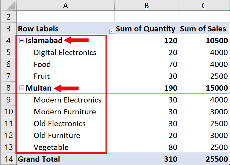
In today’s tutorial we’ll learn how to collapse all pivot table fields simultaneously. Let’s look at the dataset given below. It contains the sales data of various products from various locations. We have already created a pivot table from the data as shown above.

We can see that there are two fields or groups named Islamabad and Multan. Follow along the steps mentioned below to learn how to collapse all fields simultaneously in Excel.

Method 1: Use the context menu options

Step 1 – Collapse fields through context menu

• Select the first field of the pivot table.
• Right click from the mouse to open the context menu.
• Point to the option Expand/Collapse.
• This will open up a side menu. Choose Collapse Entire Field.
• This will collapse all fields of the pivot table as shown below.
• If you want to expand all of them back then you may press CTRL+Z or choose Expand Entire Field option from the context menu.

Method 2: Use the Pivot Table Analyze tab options

Step 1 – Collapse fields through PivotTable Analyze tab

• Click on the field in the pivot table.
• From the list of main tabs, click on the PivotTable Analyze tab.
• In the Active Field group, click on the Collapse Action button as shown below. It will collapse all the fields of the pivot table.