
How to change the legend in Excel
 By
SpreadCheaters
By
SpreadCheaters
Page last updated:
16/11/2022 |
Next review date:
16/11/2024
You can watch a video tutorial here.
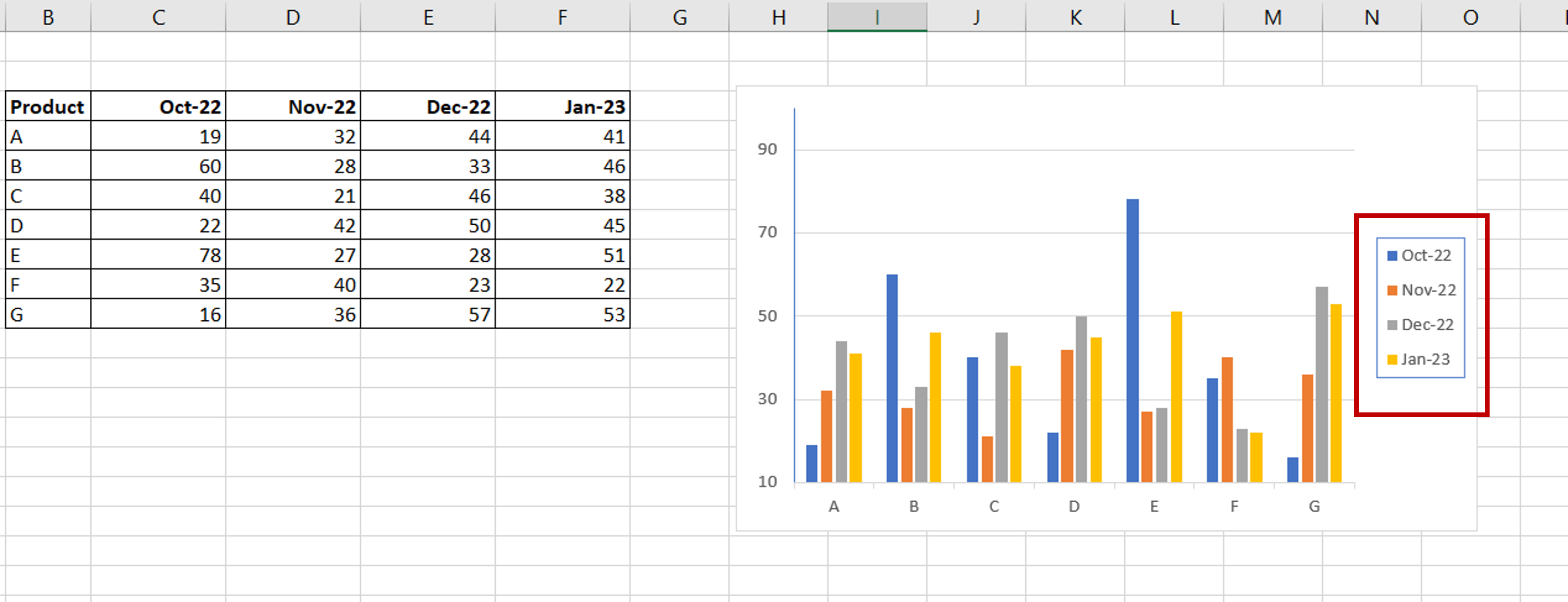
When you create a chart in Excel with multiple sets of data, it is standard practice to include a legend so that the viewer understands the data being displayed. Excel provides options to change the legend.
Step 1 – Open the Format Legend menu
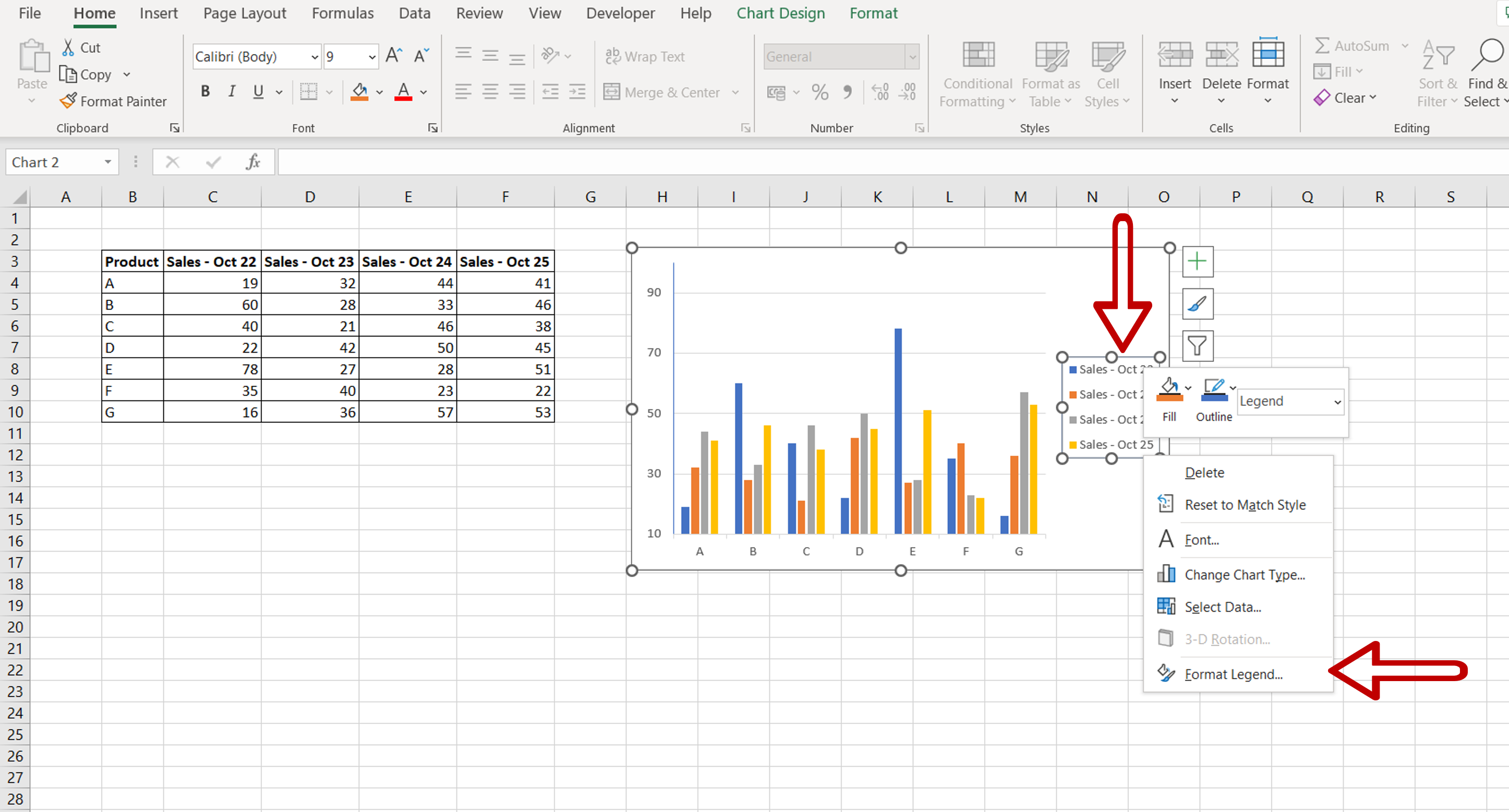
– Select the legend
– Right-click and select Format Legend from the context menu
Step 2 – Change the legend
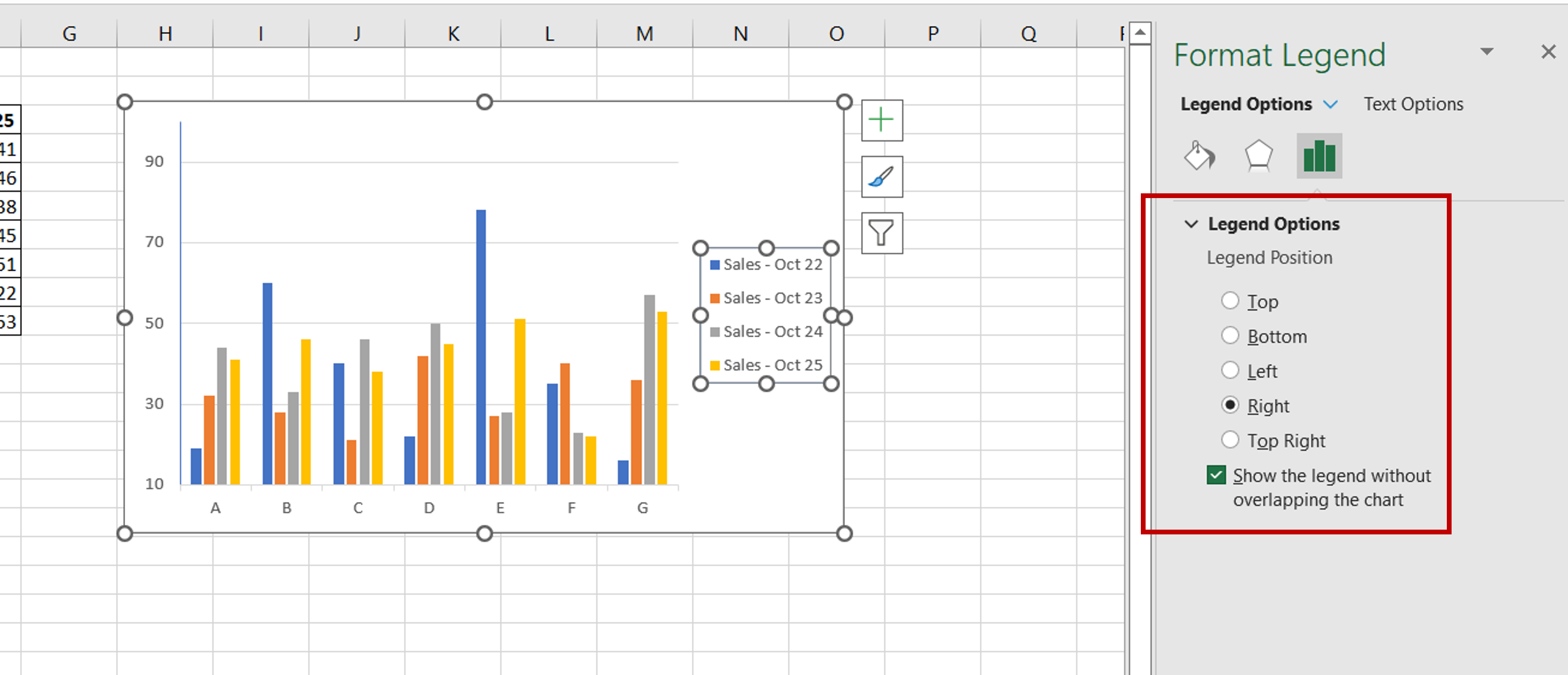
– Change the position of the legend
Step 3 – Change the text
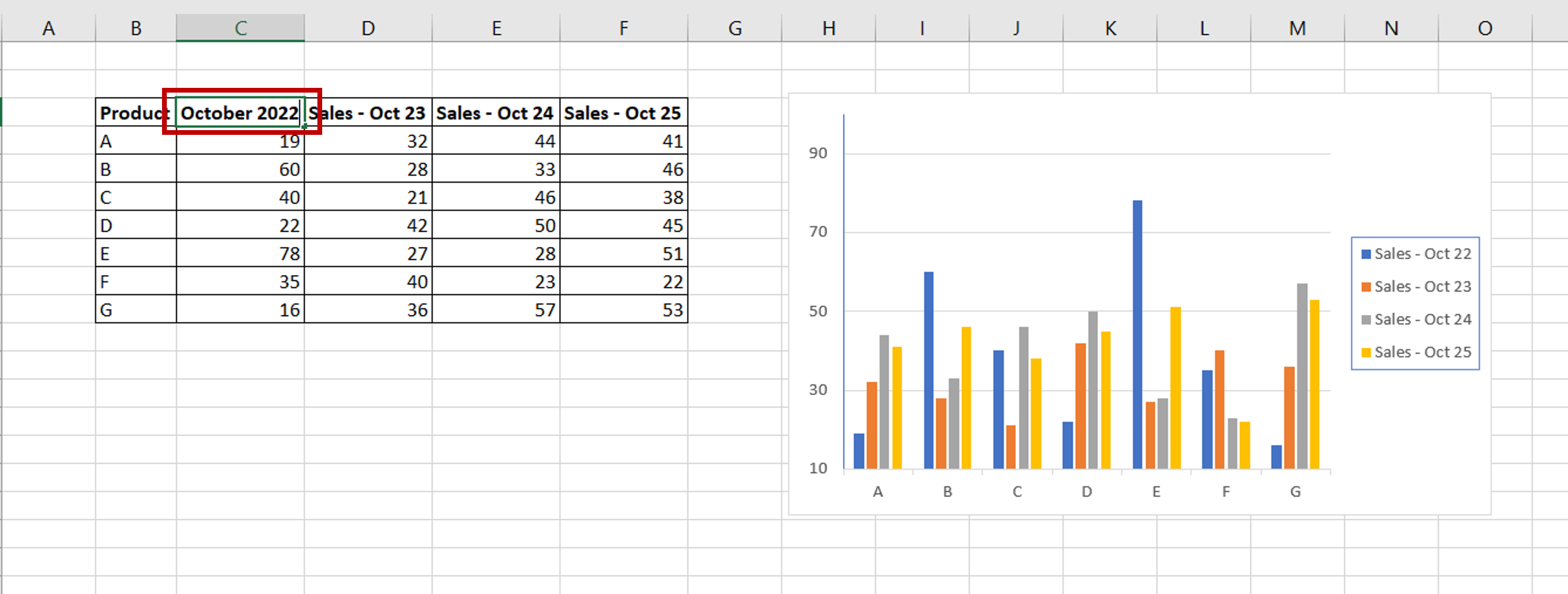
– Change the column names
Step 4 – View the result

– Check that the legend is displayed as intended
Alternate access to the Format Legend menu
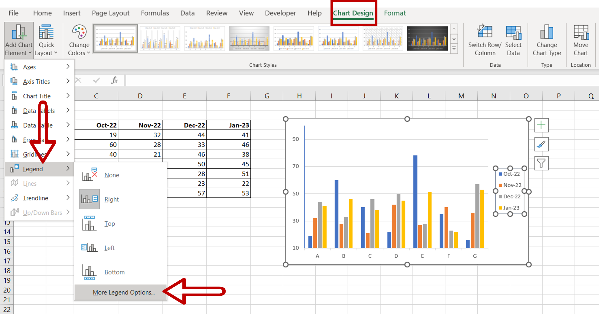
– Select the chart
– On the Chart Design menu, go to Add Chart Element > Legend > More Legend Options


