How to change row labels in a pivot table in Microsoft Excel 

In Excel, a row label is a field that is used to categorize and group data in a pivot table or a data table. Row labels are usually text-based, and they appear as the leftmost column in a pivot table. Row labels are used to organize and summarize data in a pivot table by grouping together similar data.

In this tutorial, we will learn how to change row labels in a pivot table in Microsoft Excel. It’s a common practice to change row labels in a pivot table in Excel, and there are several ways to do so. One way is to use the formula bar to edit the formula that is used for the row labels. Another way is to use the “PivotTable Analyze” tab or the Field Settings option, using this we can change the group name. 

Method 1: Using the Formulae Bar to Change the Row Label

Step 1 – Select the Row Label

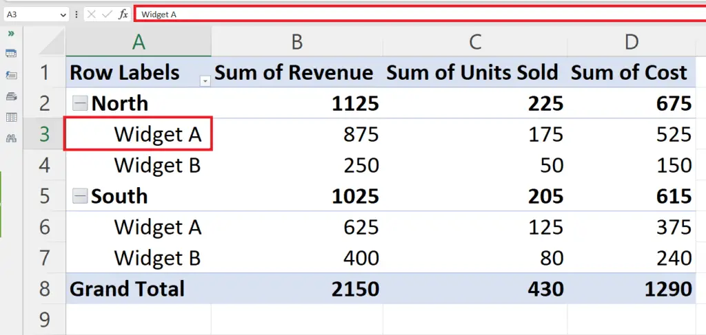
• Select the row label which you want to change in the pivot table.
• The current name of the row label will appear in the formula bar.

Step 2 – Edit the Row Label

• Edit the row label in the formula bar.

Step 3 – Press the Enter Key

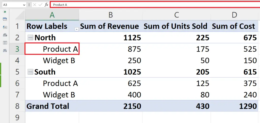
• The row label will be changed in the pivot table.

Method 2: Use the PivotTable Analyze Tab to Change the Group Name

Step 1 – Click Anywhere on the Pivot Table

• Click anywhere on the pivot table to activate the PivotTable Analyze tab.

Step 2 – Go to the PivotTable Analyze tab

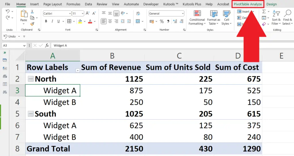
• Go to the PivotTable Analyze tab in the menu bar.

Step 3 – Select the Row Label

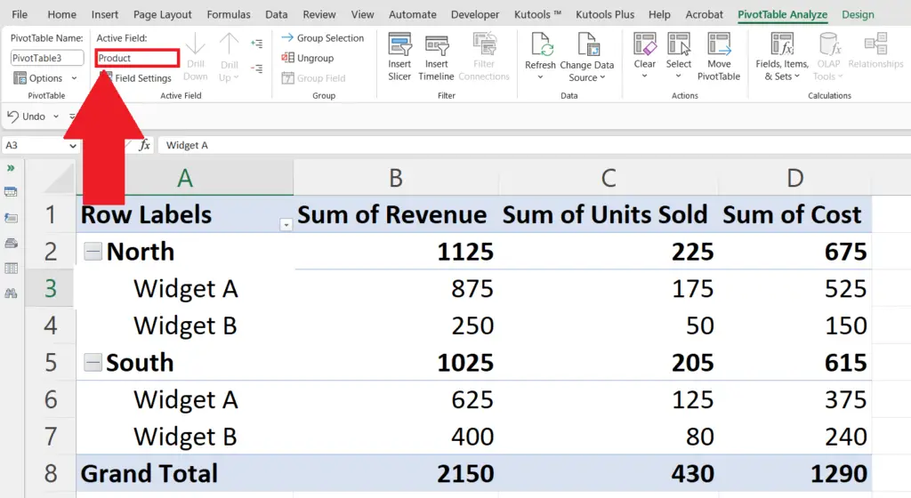
• Select the Row Label in the pivot table of which the group name is to be changed.
• The group name of the row label will appear in the Active Field text box.

Step 4 – Change the Group Name

• Change the Group name in the Active Field option.
• The group name will be changed.
• The change can be observed in the PivotTable Feilds pane.