How to change pivot table range in Excel

Pivot Table is one of the most powerful tools in Excel to analyze larger datasets keenly and extract the required data in an efficient manner. However, while working with the Pivot Table the most common issue is updating the Pivot Table range. 

In this article, we’ll learn how to update the Pivot Table using the following 3 methods.

• Update the data source manually
• Update the data source using Pivot Table Refresh function
• Convert the source data to Excel Table and use Pivot Table Refresh function

Method 1 – Update the data source manually

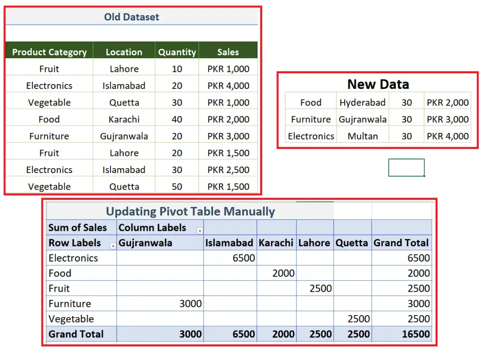
This is the manual method of updating the data source and by this method everything has to be changed manually. The dataset and the associated Pivot Table is shown below;

We want to insert the new data in the old data set and then want to update the Pivot Table as well. Let’s see how to do this by following these steps.

Step 1 – Insert the new data in old dataset

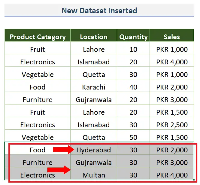
• First of all, we’ll add the new data beneath the old data set as shown below;

The new data contains the names of new locations so when we update our Pivot Table new columns will have to be added into that.

Step 2 – Go to Change Data Source option in PivotTable Analyze Tab

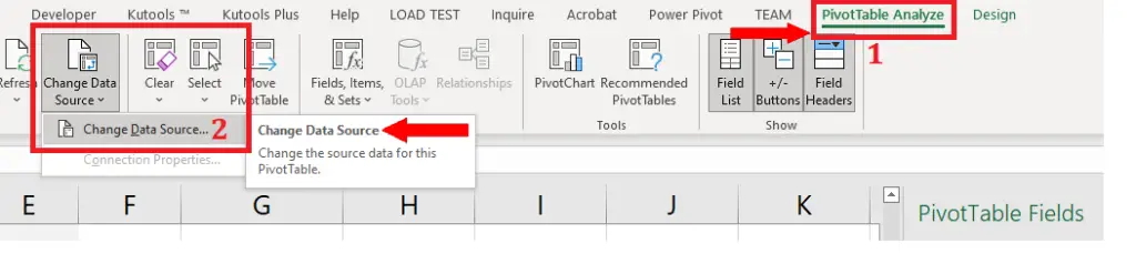
• Select a cell inside the available Pivot Table. This will enable the PivotTable Analyze tab on the list of main tabs.
• Go to the Data group, locate and click on the Change Data Source option.

Step 3 – Update the data source and update Pivot Table

• When you click on Change Data Source, a new dialog box will appear and Excel will take you to the original data source from which the Pivot Table was initially built. 
• There you need to expand the selection to include the new data values. Select them and press the OK button.
• This will update the Pivot Table automatically.

Method 2 – Update the data source using Refresh option

This is the easiest method of updating the Pivot Table range. We’ll use the same dataset and the associated Pivot Table once again. However, this method will only work if you add the new data by inserting the new rows inside the existing data. Let’s see how to do it in the following steps.

Step 1 – Insert new rows to accommodate new data

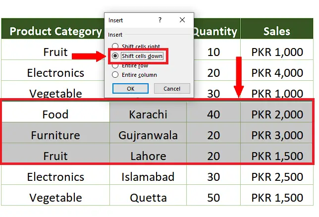
• Before inserting the new data, we’ll insert the rows inside the existing data. As we wish to add 3 more rows of data so we’ll insert 3 rows. For this select any 3 rows.
• Press CTRL + SHIFT + + together and then choose shift cells down.
• This will insert 3 blank rows inside the existing data.

Step 2 – Add the new data in the newly inserted rows

• Now add the data in the newly inserted rows by entering it manually or pasting the data in the new rows.

Step 3 – Refresh the Pivot Table to add new data

• Select a cell inside the available Pivot Table. This will enable the PivotTable Analyze tab on the list of main tabs.
• Go to Data group, locate and click on the Refresh option. This will update the Pivot Table according to the new data.

Method 3 – Convert the data source to Excel Table

In this method we’ll convert the source data to Excel Table. This will make the data source dynamic and we can then use the Refresh option of Pivot Table for updating the Pivot Table range. We’ll use the same dataset and the associated Pivot Table once again. 

Step 1 – Convert the source to Excel Table

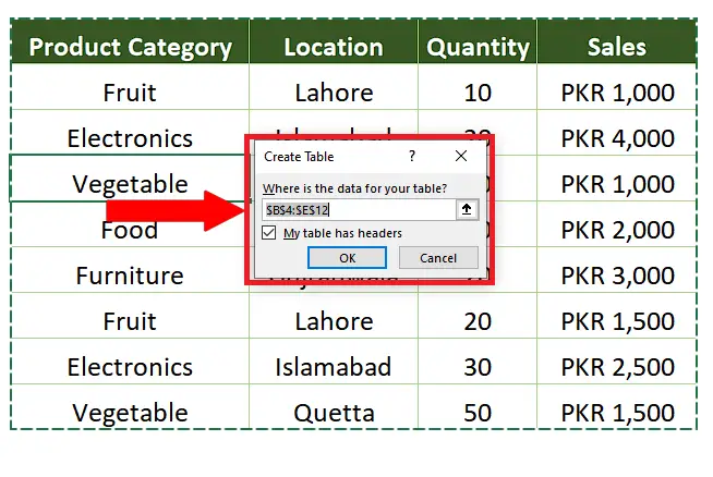
• Select any cell inside the data source and then press CTRL+T.
• This will open up a new dialog box and ask to choose the data range to convert into the Excel table. You can change the data source here or later.
• It will also ask you if your data has headers. Keep the option checked if your data include headers as well.

Step 2 – Add new data into source Table

• Now insert the new data beneath the existing data Table as shown below. Excel will automatically expand the Table and include the data into the Table.

Step 3 – Refresh the Pivot Table to add new data

• Select a cell inside the available Pivot Table. This will enable the PivotTable Analyze tab on the list of main tabs.
• Go to the Data group, locate and click on the Refresh option. This will update the Pivot Table according to the new data.