How to change legend names in Excel

You can watch a video tutorial here.

Charts are a great way to visualize data and Excel provides several options for creating charts and formatting them. When you create a chart in Excel with multiple sets of data, it is a good practice to include a legend so that the viewer understands the data being displayed. Excel provides two ways in which the legend names can be changed:

1. Change the name in the underlying dataset
2. Change the name of the series 

Option 1 – Change the underlying dataset

Step 1 – Change the first name

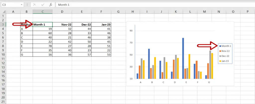
• Go to the dataset on which the chart is built
• Change the first column name
• Press Enter
• Check that the legend is updated with the new name

Step 2 – Change all the names

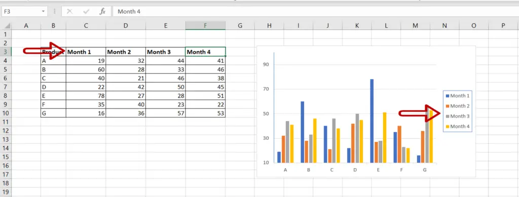
• Change the other names
• The legend is updated with the new names

Option 2 – Change the name of the series

Step 1 – Open the Select Data Source box

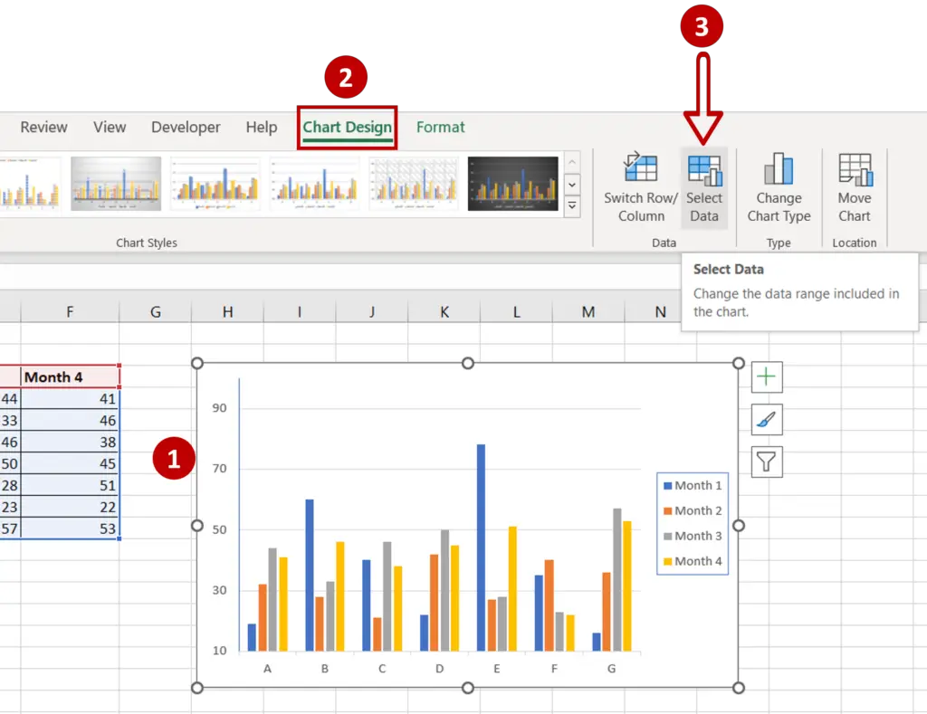
• Select the chart to summon the Chart Design  menu option
• Go to Chart Design > Data
• Click on Select Data

Step 2 – Open the Edit Series box

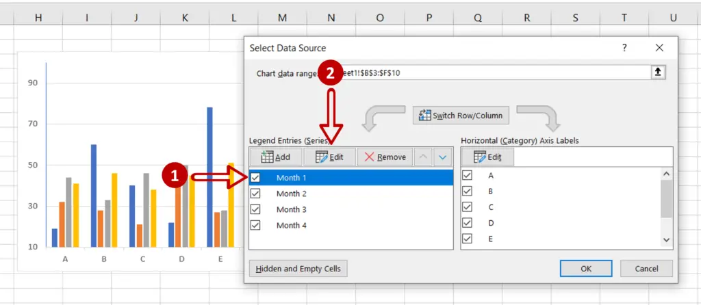
• Under Legend Entries (Series), select ‘Month 1’
• Click Edit

Step 3 – Change the first series name

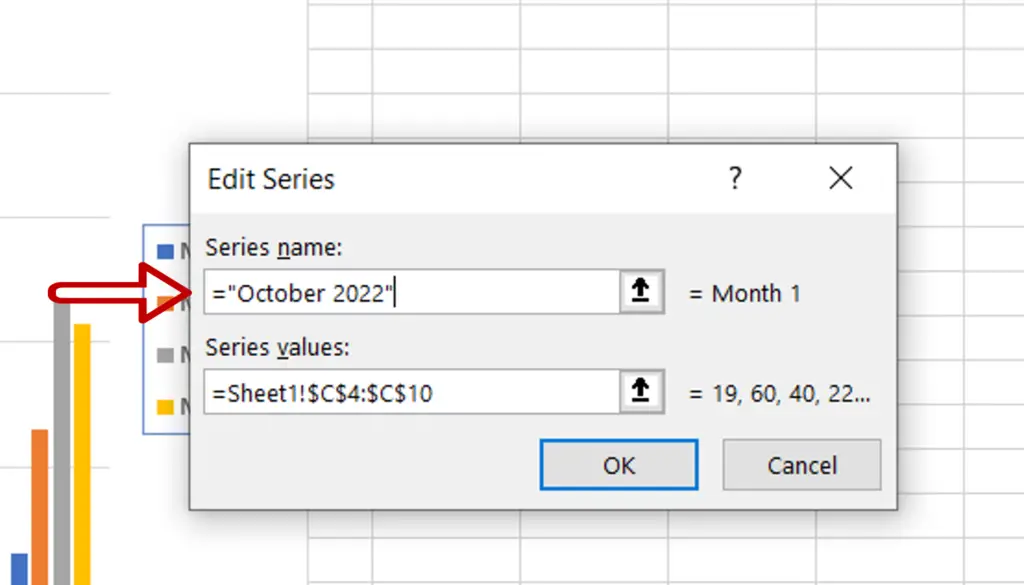
• Under Series name enter:

=”October 2022”

• Click OK

Step 4 – Change all the series names

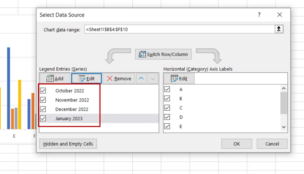
• Repeat Step 3 for all the series names:
  • Month 2 =”November 2022”
  • Month 3 =”December 2022”
  • Month 4 =”January 2023”
• Click OK to close the Select Data Source box

Step 5 – Check the result

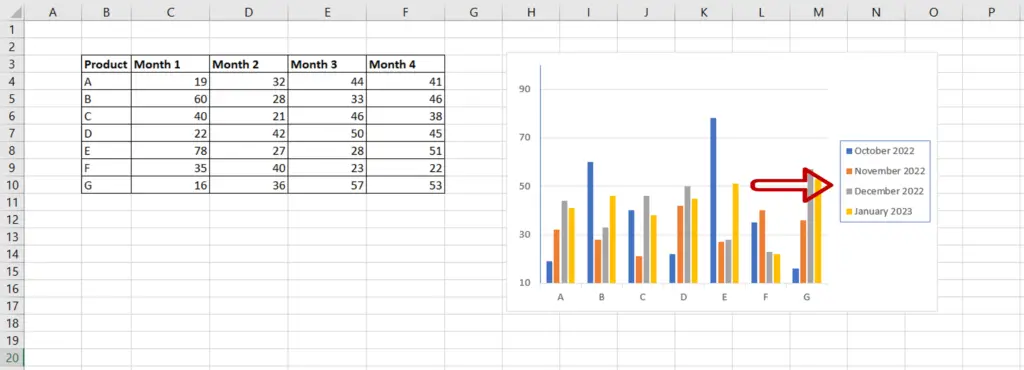
• The names have changed in the legend without changing the names in the underlying dataset