How to change date format in pivot table in Excel

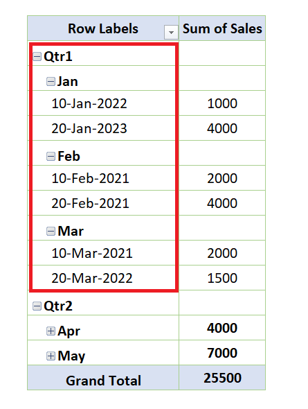
In today’s tutorial, we have the following pivot table dataset containing sales amount on dates and total sale in ungrouped form. We’re going to use this dataset to change the format of dates in the pivot table. Consider this following dataset above as an example to learn today’s tutorial.

The problem with changing the date format of pivot table is that when the dates are grouped together, you can’t change the date format. Even if you try to change the format the changes won’t take effect. To overcome this issue let’s explore the steps mentioned below.

The default date format in Excel may not be easy to read or understand. Pivot tables are used to summarize and aggregate data. Standardizing the date format in a pivot table ensures consistency and reduces the risk of errors in analysis and reporting. Changing date formats in pivot tables in Excel can improve readability, sorting and filtering, consistency, and aggregation of data.

Step 1 – Ungrouping the data in pivot table

– This is for the data that is already grouped.
– Select any cell in which date is present.
– Right click on it.
– Select the Ungroup option.

Step 2 – Grouping data again to change the date format

– Select any cell in which date is present.
– Right click on it.
– Select the Group option.
– A pop-up box will appear.
– Select any format you want from it, e.g., we’re going to select days, months and years.
– Click on OK.
– Now, your data will be converted to grouped data according to the chosen format.