
How to categorize data in Microsoft Excel
 By
SpreadCheaters
By
SpreadCheaters
Categorizing data in Excel is an essential process that helps to organize, sort, and analyze large datasets efficiently. It allows users to group data by various categories such as date, product, location, or any other relevant factor to facilitate better analysis and reporting. The main uses of categorizing data in Excel include easy organization, efficient analysis, improved decision-making, enhanced reporting, and improved accuracy.
In this tutorial, we will learn how to categorize data in Microsoft Excel. To categorize data in Excel, you can use various tools such as filters, XLOOKUP or VLOOKUP, and the IF function, etc. We will use the XLOOKUP function to categorize data into columns.
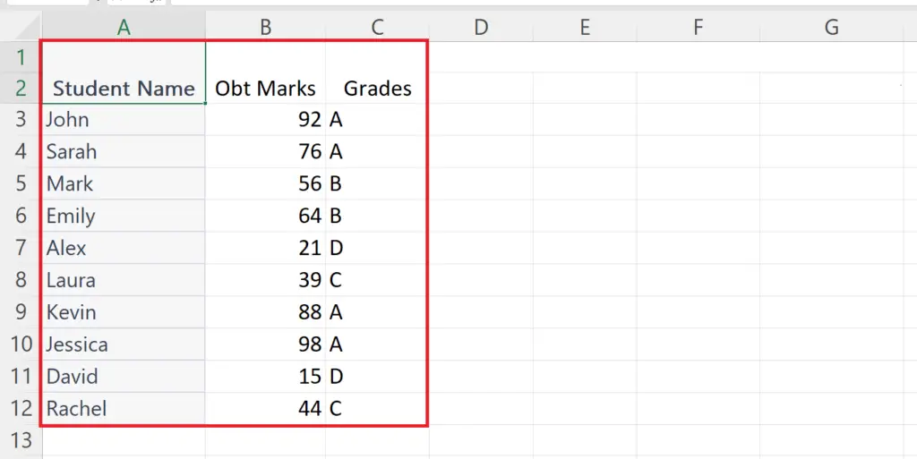
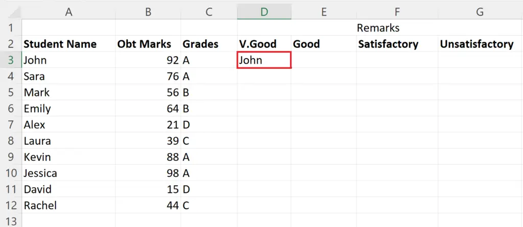
Currently, we have a data set representing the obtained marks and grades of 10 students. We want to categorize students into remarks columns according to obtained grades i.e. V. Good for grade A, Good for grade B, Satisfactory for grade C, and Unsatisfactory for grade D. We will use the XLOOKUP and IF function to categorize the students into columns on the bases of their grades.
Method 1: Categorizing Data using the XLOOKUP Function
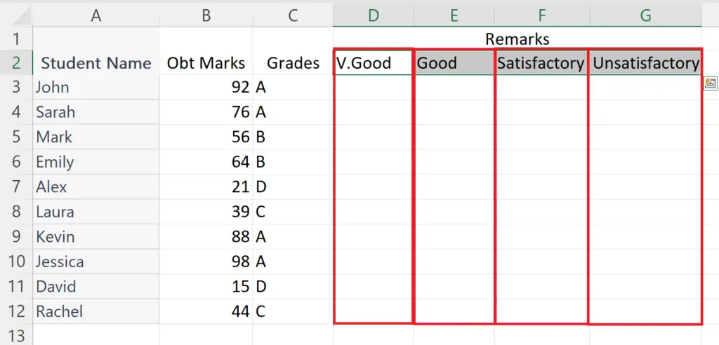
Step 1 – Make a Column for Each Category

- Make a column for each category i.e.V.Good, Good, Satisfactory, and Unsatisfactory.
Step 2 – Select the First Cell of a Category
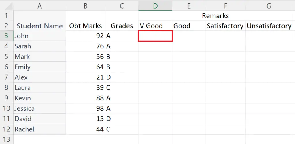
- Select the first cell of the column for the first category i.e. V.Good.
Step 3 – Place an Equals Sign and Enter the XLOOKUP Function
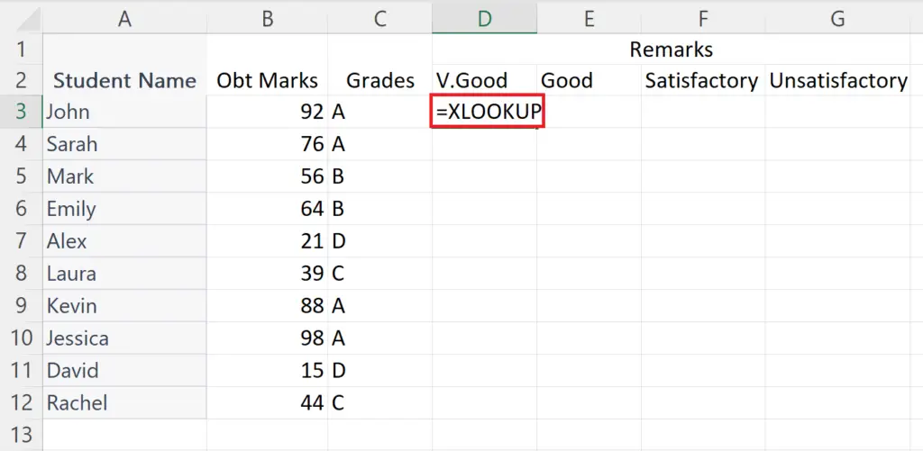
- Place an Equals sign in the selected cell.
- Enter the XLOOKUP function.
Step 4 – Enter the Lookup Value
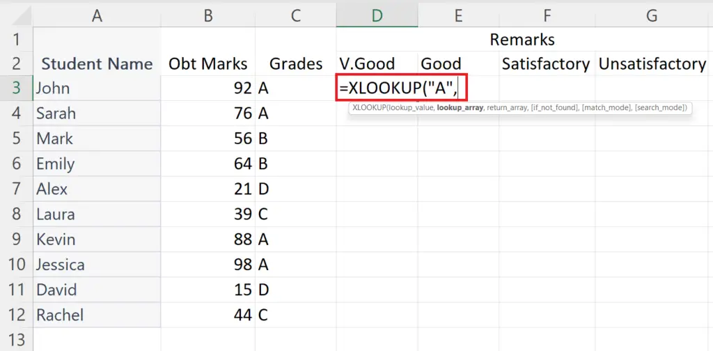
- Enter the Lookup value in the XLOOKUP function i.e. the categorizing factor ( A ).
- Place a comma.
Step 5 – Enter the Lookup Array
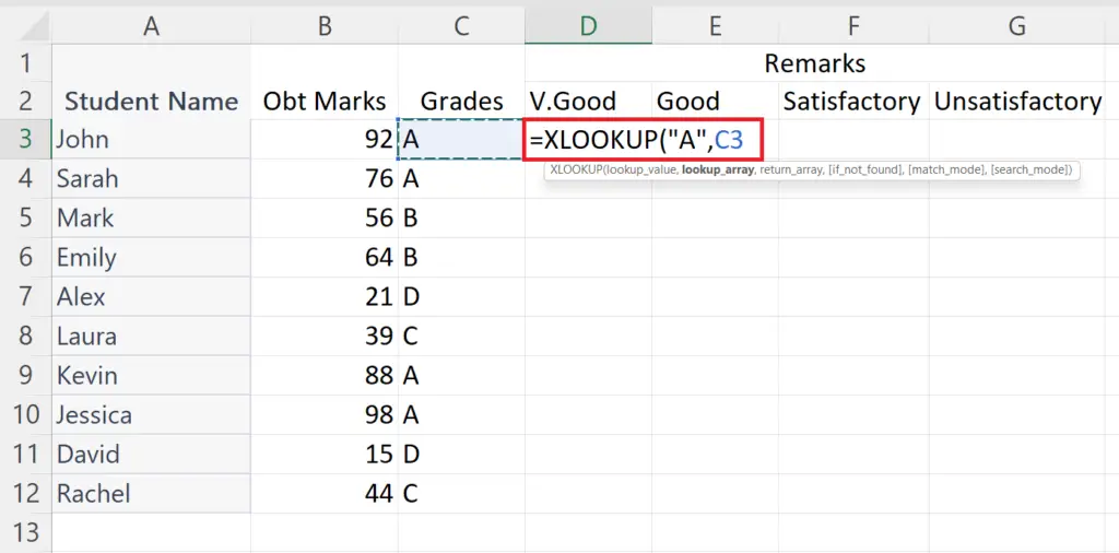
- Enter the Lookup array i.e. the range of cells or a cell containing the Lookup value.
- Place a Comma.
Step 6 – Enter the Return Array
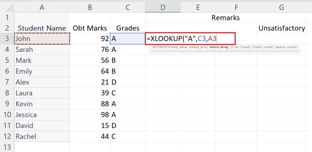
- Enter the Return array i.e. the range of cells or a cell containing the value to be returned.
Step 7 – Enter the [If_not_found value] Value
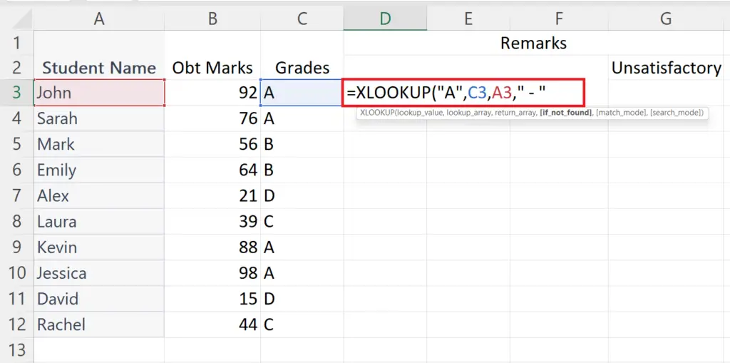
- Enter the [If_not_found value] value i.e. the value to be returned if no match is found.
- I.e. “ – “
Step 8 – Enter the Match Mode
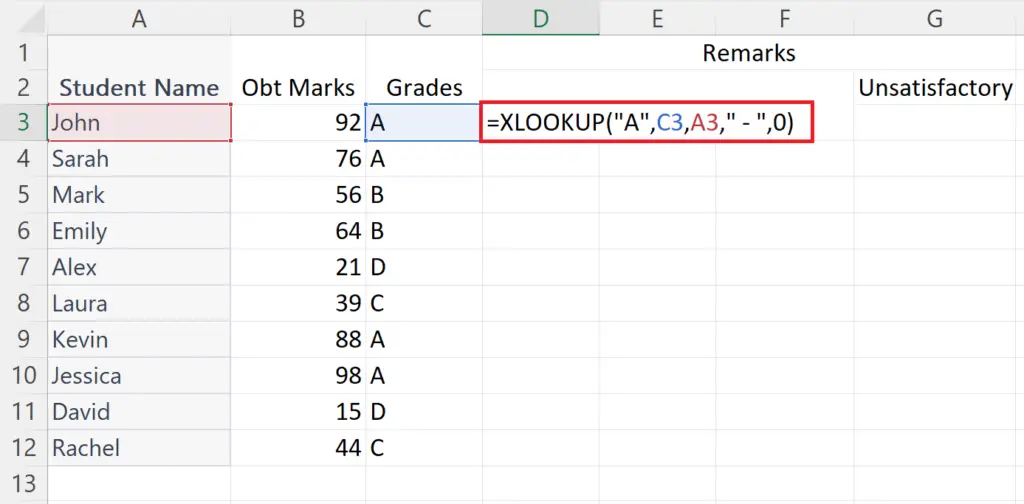
- Enter the Match mode i.e. 0,-1,1, or 2.
Step 9 – Press the Enter Key
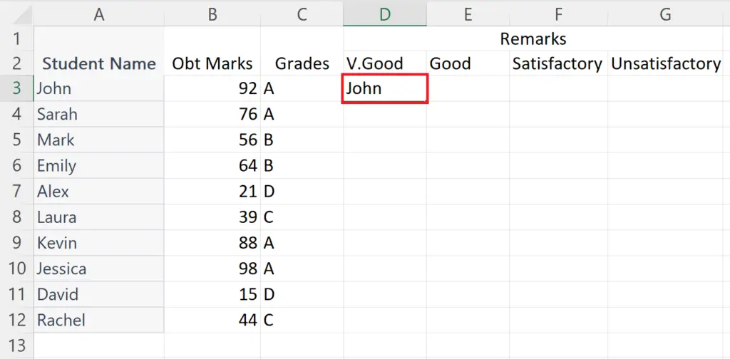
- Press the Enter key.
- The function will return the name of the first student with Grade A.
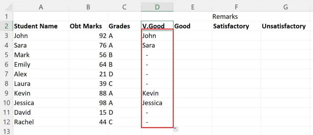
Step 10 – Use the Fill Feature to Apply the Function on the Complete Column

- Use the Fill feature to Apply the Function on the complete column.
- All the students having an A grade will be listed in the column.
Step 11 – Apply the XLOOKUP Function in the First Cell of Each Column
- Repeat the same steps to apply the XLOOKUP function in the first cell of each column by replacing the Lookup value i.e.B, C, D.
Step 12 – Use the Fill Feature to Apply the Function on the Complete Column of Each Category
- Use the Fill feature to apply the function on the complete column of each category.
- In this way, all the students will be categorized into the Remarks columns according to the categorizing factor i.e the grades.
Method 2: Categorizing Data using the IF Function
Step 1 – Make a Column for Each Category
- Make a column for each category i.e.V.Good, Good, Satisfactory, and Unsatisfactory.
Step 2 – Select the First Cell of a Category

- Select the first cell of the column for the first category i.e. V.Good.
Step 3 – Place and Equals Sign and Enter the IF Function
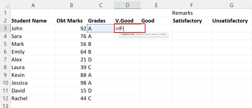
- Place and Equals Sign in the blank cell.
- Enter the IF function.
Step 4 – Enter the Logical Test
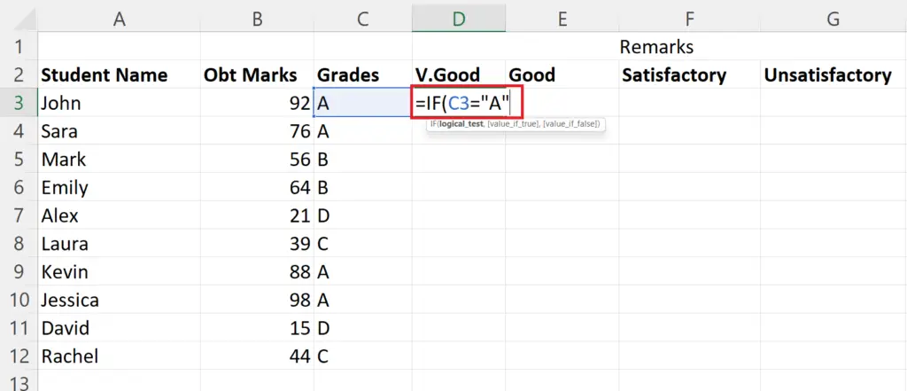
- Enter the logical test based on which you want to categorize the data.
- Here we want to check whether the Grade is A.
- So the logical test will be:
C2= “A”
- C2 is the cell containing the value to be checked and “A” is the value required.
Step 5 – Enter the If True Value
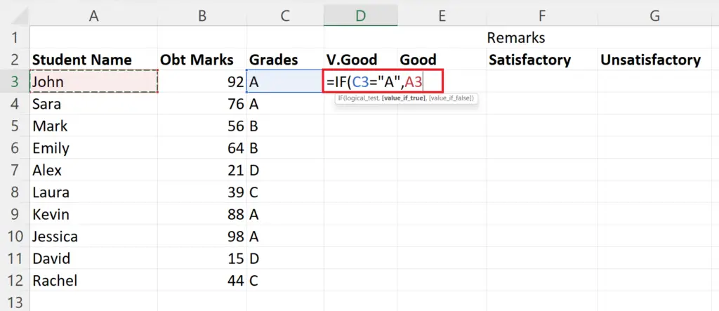
- Place a comma.
- Enter the value which you want to return if the tested value is true.
- Here we will enter A2 as the if true value. A2 is the cell containing the name of the student which is to be printed.
Step 6 – Enter the If False Value
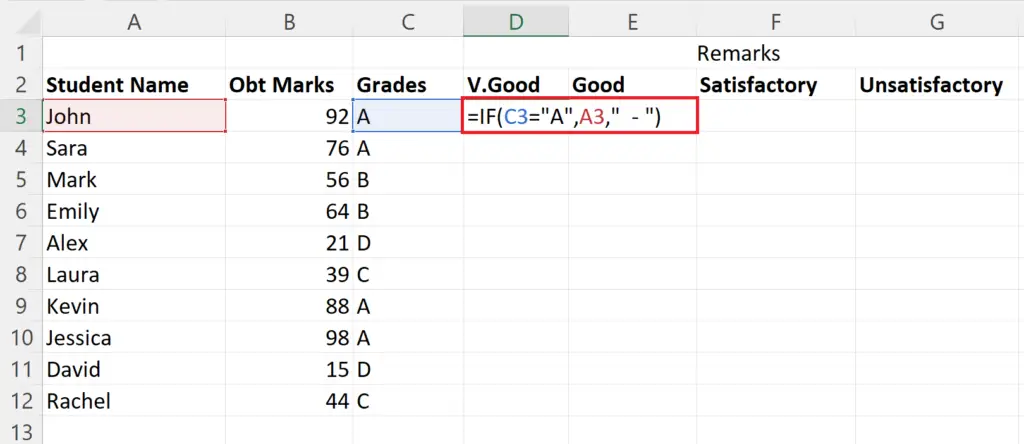
- Place a comma.
- Enter the value which is to be returned if the tested value is false i.e. “ – “.
Step 7 – Press the Enter Key.
- Press the Enter key to get the results.
Step 8 – Use the Fill Feature to Apply the Function on the Complete Column
- Use the Fill feature to Apply the Function on the complete column.
- All the students having an A grade will be listed in the column.
Step 9 – Apply the IF Function on Each Column
- Apply the IF function on the first cell of each column in a similar way by replacing the required value i.e. B, C, D.
Step 10 – Use the Autofill Feature on Each Column
- Use the Autofill feature separately on each column to categorize the data in each column.
Method 3 – Categorizing Data Using the VLOOKUP Function
The VLOOKUP function can be utilized for categorizing data. Its syntax is :
VLOOKUP(lookup_value, table_array, col_index_num, [range_lookup])
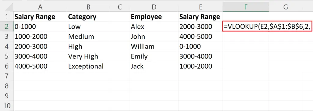
For this we have a separate dataset. In the provided dataset, a table with the range A1:B6 represents categories based on salary. The list of employees along with their salary range is present in D1:E6. Our objective is to classify them according to their salary range using the table, and to accomplish this, we will use column F.
Step 1 – Select a Blank Cell
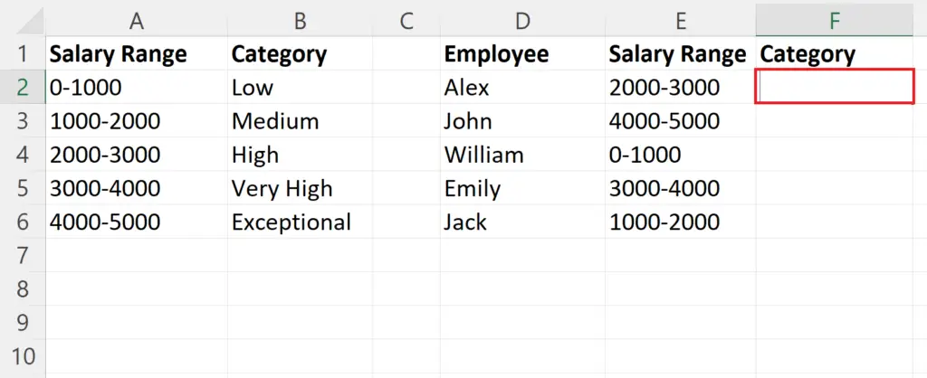
- Select a blank cell in the column where you want to categorize the data.
Step 2 – Place an Equals Sign and Enter the VLOOKUP Function
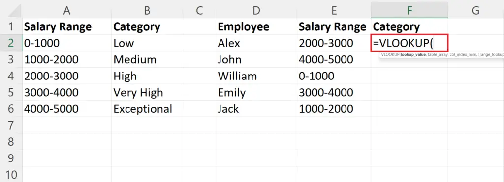
- Place an Equals sign and enter the VLOOKUP function.
Step 3 – Enter the Lookup Value
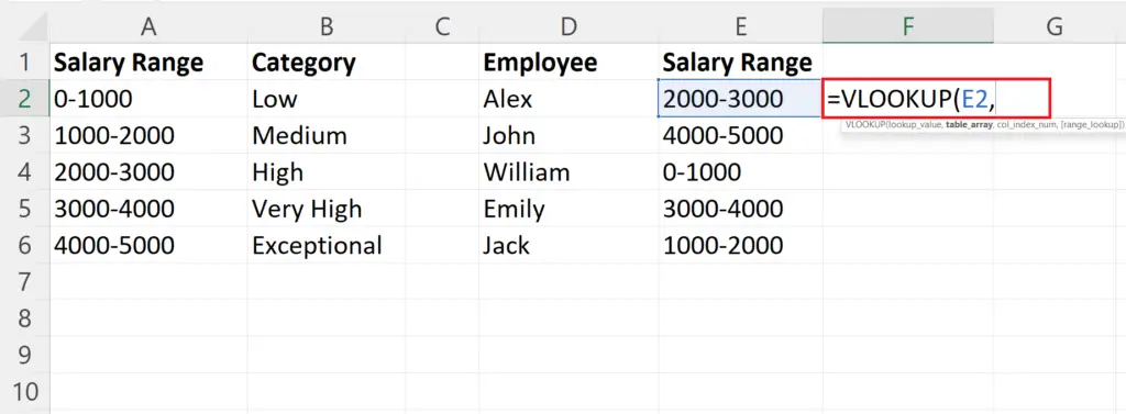
- Enter the first argument i.e. the lookup value.
- Place a comma ( , ) .
Step 4 – Enter the Range of the Table Array
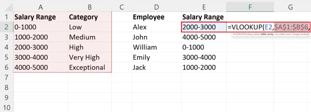
- Enter the range of the table array.
- Place a comma ( , ).
Step 5 – Enter the Column Index
- Enter the index of the column containing the value to be returned.
- Here the column index will be 2 as the return values are present in the second column of the table.
- Place a comma ( , ) .
Step 6 – Enter the Range of Lookup
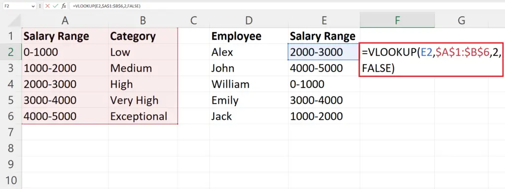
- Enter the method of lookup i.e. True – for approximate match , False – for exact match.
Step 7 – Press the Enter Key
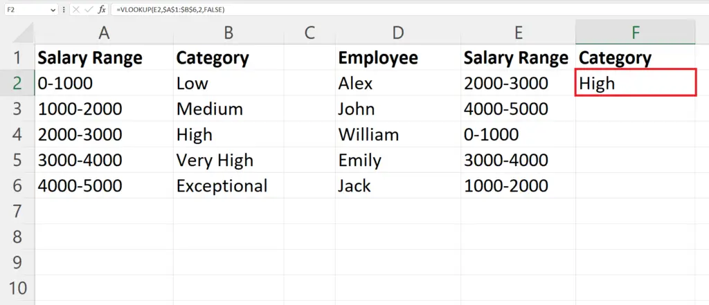
- Press the Enter key to get the value.
Step 8 – Use Autofill to apply the VLOOKUP Function on Each Row
- Use the Autofill feature to apply the VLOOKUP function on each row of the column.


