
How to calculate Y intercept in Excel
 By
SpreadCheaters
By
SpreadCheaters
When working with data in Excel, understanding the relationship between variables is crucial for data analysis and modeling. One essential aspect of linear regression is determining the y-intercept, which represents the value of the dependent variable (y) when the independent variable (x) is zero. Calculating the y-intercept can provide valuable insights into the starting point of a linear relationship. In this blog post, we will guide you through the process of calculating the y-intercept in Excel, enabling you to perform accurate linear regression analysis and make informed decisions based on your data.
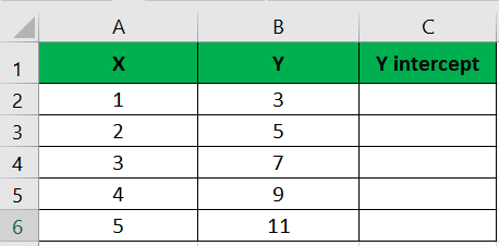
The dataset is a small and randomly generated set of values for two variables, X and Y. It was likely created for educational or illustrative purposes to demonstrate data analysis techniques. The X variable represents the independent variable, while the Y variable represents the dependent variable. The dataset allows for practicing and understanding concepts such as linear regression and calculating the y-intercept using Excel.
Method – 1 “linear regression analysis” or “least squares regression analysis.”
The method involves using Excel’s LINEST function to calculate the y-intercept of a linear regression line. By providing the y-values and x-values as inputs, the function performs a regression analysis and returns an array of values, including the y-intercept. This method allows for determining the starting point of the regression line on the y-axis based on the given dataset.
Step – 1 Enter the formula in an empty cell
- Select an empty cell; choose a cell where you want to display the result.
- Use the LINEST function: In the selected cell, enter the formula “=LINEST(y-values, x-values)“.
- Replace “y-values” and “x-values” with the appropriate cell references: Select the range of cells containing the Y-values for “y-values” and the range of cells containing the X-values for “x-values“.
Step – 2 Press Ctrl + Shift + Enter
- Press Ctrl + Shift + Enter; Instead of just pressing Enter, use the Ctrl + Shift + Enter keyboard shortcut to indicate that you’re entering an array formula.
- Extract the y-intercept value; the result will be an array of values. The y-intercept will be located in the first cell of the resulting array.
Method – 2 Calculating Y intercept from statistical Formulas
The method involves using Microsoft Excel to calculate the y-intercept using linear regression analysis. It requires inputting X and Y values, selecting the appropriate function, and letting Excel perform the calculation. The result is the y-intercept value based on the provided data.
Step – 1 Open LINEST dialog box
- Navigate to the “Formulas” tab in the Excel ribbon
- Click on the “More Functions” button.
- From the dropdown menu, choose the “Statistical” category and scroll down to select the “LINEST” formula.
Step – 2 Select the Entire columns of X and Y values
- Click on the “Function arguments” button located next to the “Known Y’s” field. Select the entire column of Y values and press “Enter“. Repeat the same process for the “Known X’s” field by selecting the entire column of X values. Click “OK” to proceed.
- Excel will then compute the y-intercept using the provided X and Y values, and the result will be displayed.
Conclusion:
In conclusion, calculating the y-intercept in Excel using linear regression analysis is a valuable tool for understanding the relationship between variables and making predictions based on the regression model. Determining the y-intercept provides insights into the starting point of the regression line on the y-axis and helps interpret the behavior of variables when the independent variable is zero. Excel’s functionality simplifies the process, making it accessible and convenient for various fields, including economics, finance, science, and engineering. By utilizing this method, one can make data-driven decisions and gain a deeper understanding of the variables’ linear relationship.


