How to calculate trend analysis in Microsoft Excel 

Trend analysis in Excel is a method of analyzing and forecasting data over time. It helps identify patterns, trends, and relationships between variables, which can be used to make informed decisions about future trends. 

In this tutorial, we will learn how to calculate tren analysis in Microsoft Excel. Excel offers several tools and features for trend analysis, including the Trend function and the trendline chart element. These tools can be used to identify patterns, trends, and relationships in your data and make informed decisions about future trends.

An example could be analyzing the sales and cost figures of a firm over a decade using the Trendline and Trend features to calculate trend analysis.

Method 1: Using the TRENDLINE Feature

Step 1 – Select the Data

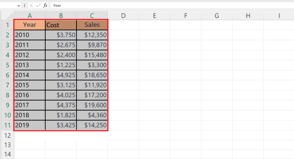
• Select the range of cells containing the data i.e. Sales and Cost.

Step 2 – Go to the Insert Tab

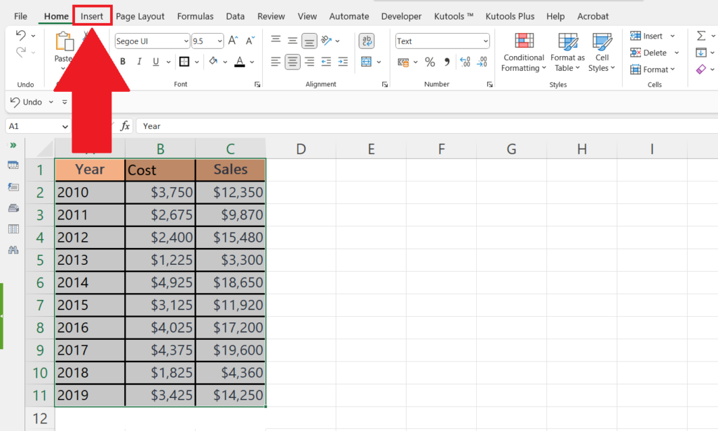
• Go to the Insert tab in the menu bar.

Step 3 – Create a Chart 

• Create a chart using the Charts section.

Step 4 – Select the Chart and Click on the Chart Elements 

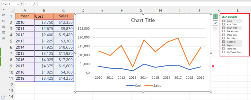
• Select the chart.
• A green plus sign (Chart Elements) would appear on the top right corner of the chart.
• Click on the Chart Elements option i.e. the plus sign.
• The Chart Elements list will appear.

Step 5 – Enable the Trendline

• Enable the Trendline feature by checking the box prior to the Trendline option.
• Select the data header for which you want to create the trend line.

Method 2: Using the TREND Function

We will calculate the trend for the cost using the TREND function.

Step 1 – Select a Blank Cell and Place an Equals Sign

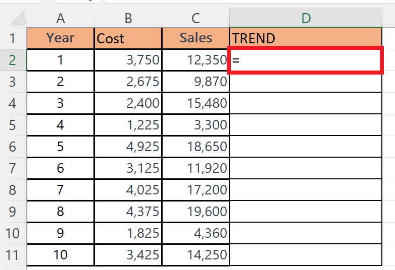
• Select a blank cell where you want to calculate the trend.
• Place an Equals Sign.

Step 2 – Enter the Trend Function

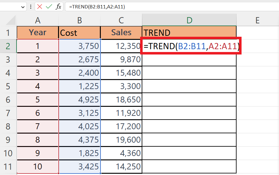
• Enter the TREND function.
• The syntax of the TREND function is;

            TREND( B2:B11 , A2:A11 )

• The first argument B2:B11 is the range containing the dependent variables.
• The second argument i.e. A2:A11 is the range containing the independent variables.

Step 3 – Press the Enter Key

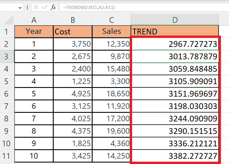
• Press the Enter key. 

Step 4 – Forecast Cost for the Next Two Years

• We can utilize the TREND function to forecast value for the next years also.
• This can be done by entering the TREND formulae in the cell where the forecast value is to be placed.
• The syntax would be:

              TREND( B2:B11 , A2:A11,A12:A13 )

• Where the third argument A12:A13 has the new independent variables for which the dependent values are to be forecasted.