
How to calculate the Sharpe ratio in Excel
 By
SpreadCheaters
By
SpreadCheaters
You can watch a video tutorial here.
To calculate the Sharpe ratio in Excel, you need to have the following information in place:
- The rate of return of the portfolio for a given period
- The risk-free rate of return for the same period
The Sharpe ratio is used to evaluate the relationship between risk and return for a portfolio. Excel does not have a function for this calculation but you can create the formula for the ratio in Excel. The formula for calculating the Sharpe ratio is:
– Sharpe ratio = (return of the portfolio – risk-free return) / standard deviation of the excess returns of the portfolio
>The return of the portfolio is taken from the actual performance of the portfolio
>Risk-free return is the return of an investment that is risk-free such as government bonds
>The standard deviation of the portfolio will be computed using the STDEV.P() function
– STDEV.P() function: returns the standard deviation of a set of numbers
>Syntax: STDEV.P(range of numbers)
Step 1 – Compute the excess returns
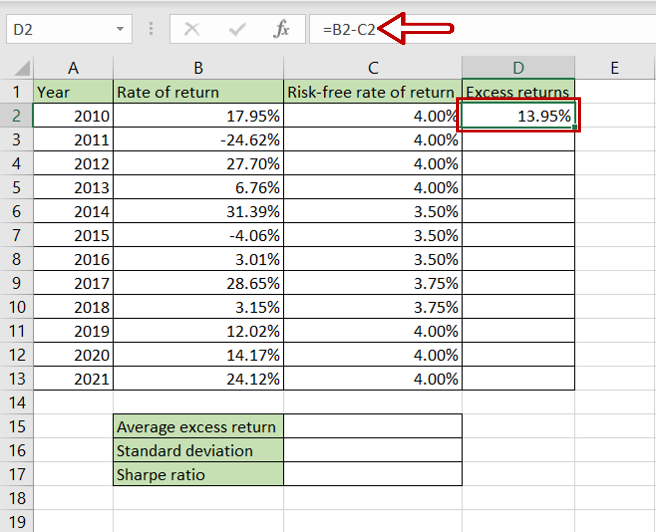
– Select the cell where the result is to appear
– Type the formula using cell references:
= Rate of return – Risk-free rate of return
– Press Enter
Step 2 – Copy the formula
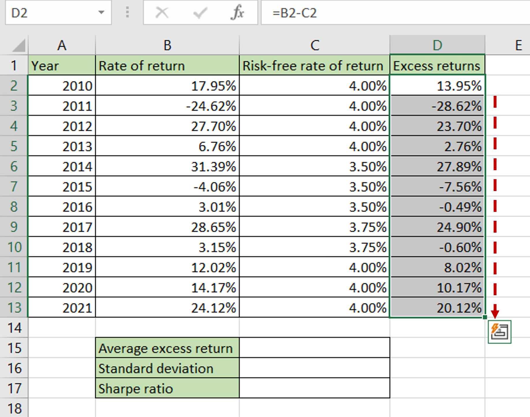
– Using the fill handle from the first cell, drag the formula to the remaining cells
OR
a) Select the cell with the formula and press Ctrl+C or choose Copy from the context menu (right-click)
b) Select the rest of the cells in the column and press Ctrl+V or choose Paste from the context menu (right-click)
Step 3 – Compute the average excess returns
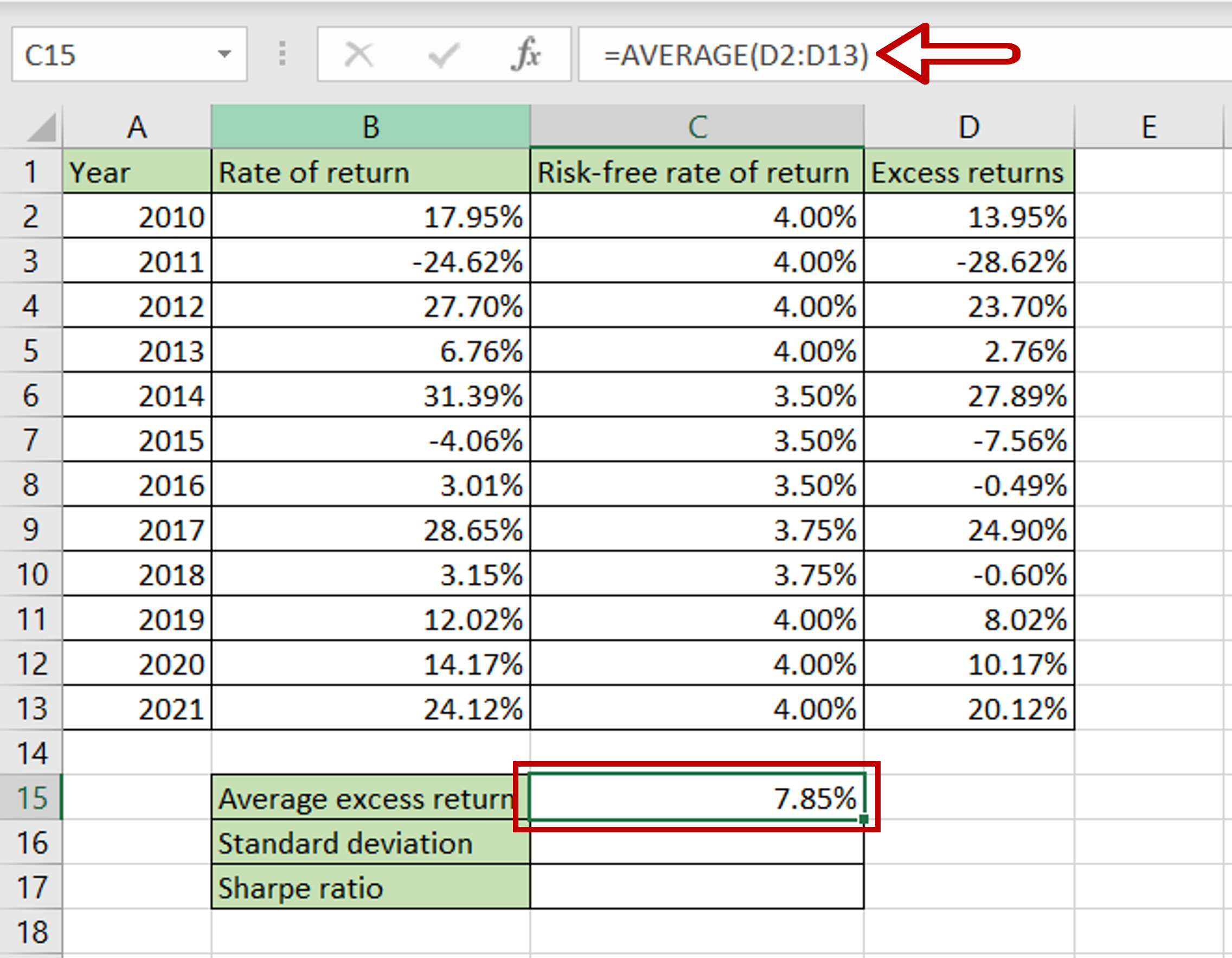
– Select the cell where the result is to appear
– Type the formula using cell references:
= AVERAGE (range of Excess returns)
– Press Enter
Step 4 – Compute the standard deviation
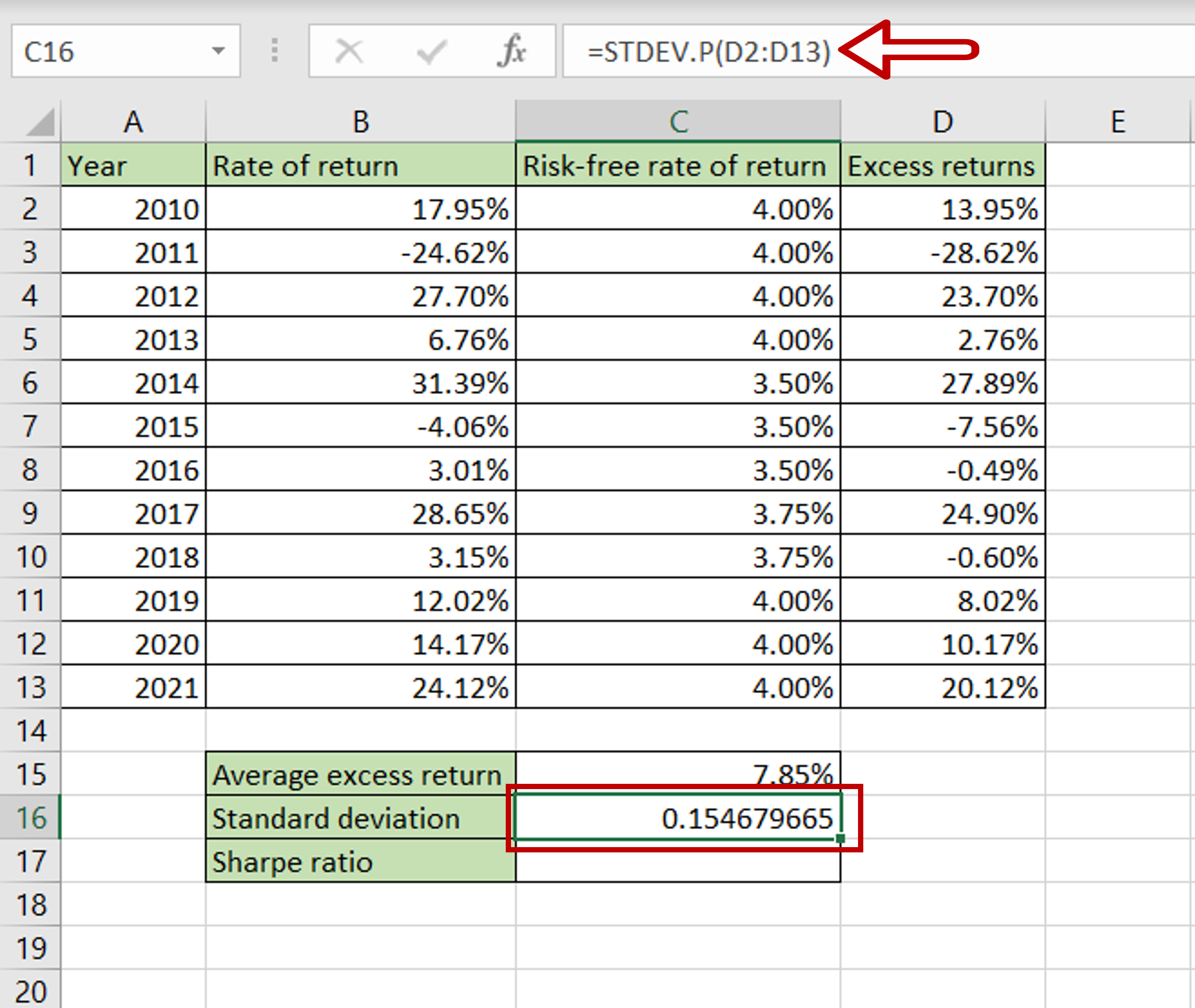
– Select the cell where the result is to appear
– Type the formula using cell references:
= STDEV.P(range of Excess returns)
– Press Enter
Step 5 – Format the standard deviation as percentage
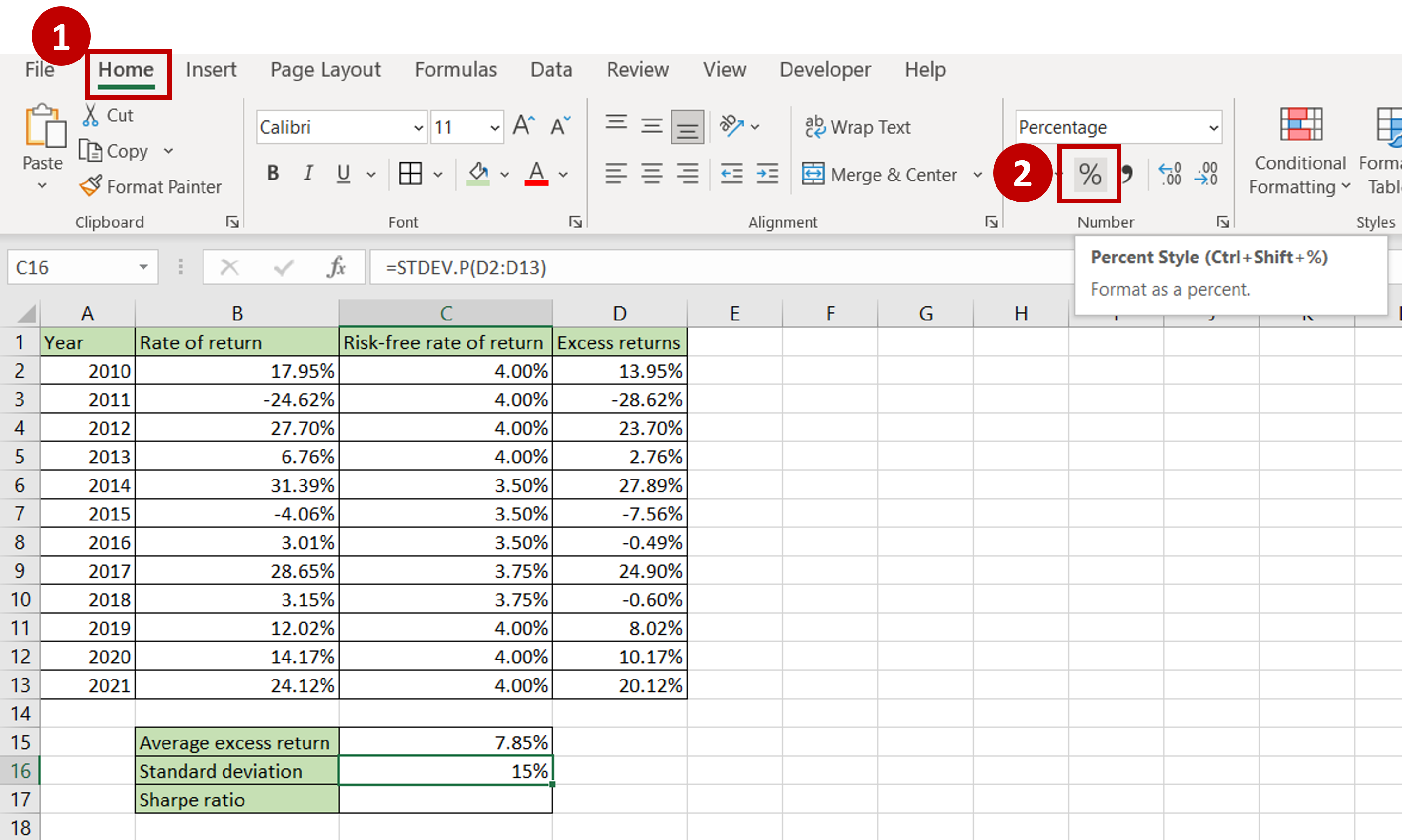
– Select the cell with the value
– Go to Home > Number
– Click on the percentage sign (%)
OR
Open the Format Cells window (Home > Number and click on the arrow to expand the menu OR Right-click and select Format Cells from the context menu OR Go to Home > Cells > Format > Format Cells) and select Number > Percentage and click OK
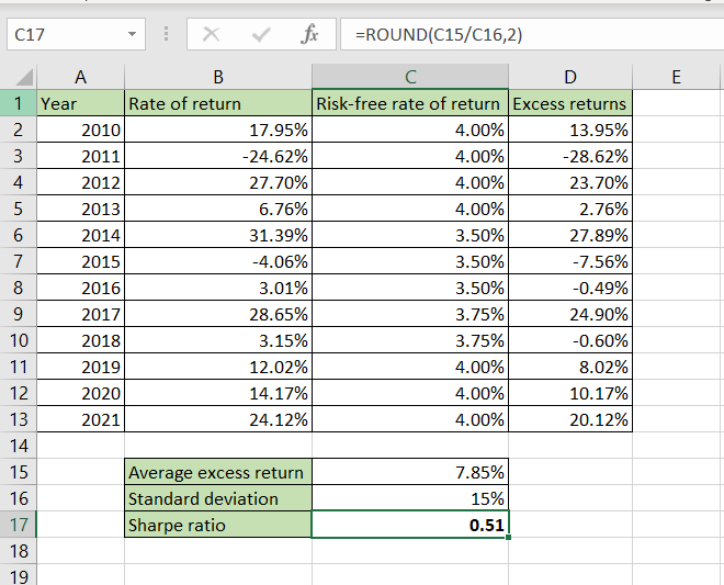
Step 6 – Compute the Sharpe ratio
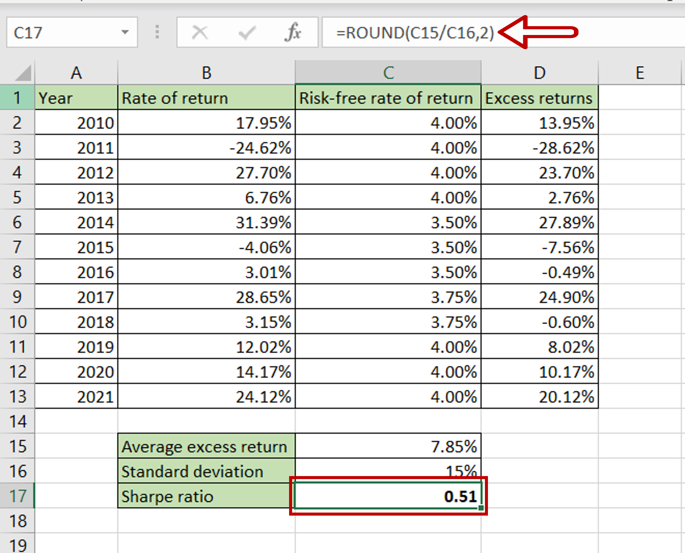
– Select the cell where the result is to appear
– Type the formula using cell references:
= ROUND(Average excess return/ Standard deviation,2)
Note: The ROUND() function is used to display 2 decimal places
Press Enter


