
How to calculate the percentage of a total in Excel
 By
SpreadCheaters
By
SpreadCheaters
You can watch a video tutorial here.
Excel is frequently used for calculations and supports all basic mathematical operations. Frequently, you will need to calculate the percentage of a total. In this example, we will look at foreign tourists’ arrival in India in the year 2020. The number of tourists from each country is given and we will compute each number as a percentage of the total to see from which country there was the highest number of tourists. To do so in, we will use the mathematical formula:
(Number/total)*100
In Excel, we just need to divide the numbers and then format the cell as a percentage. This will multiply the value by 100 and add a percentage sign (%).
Step 1 – Create the formula
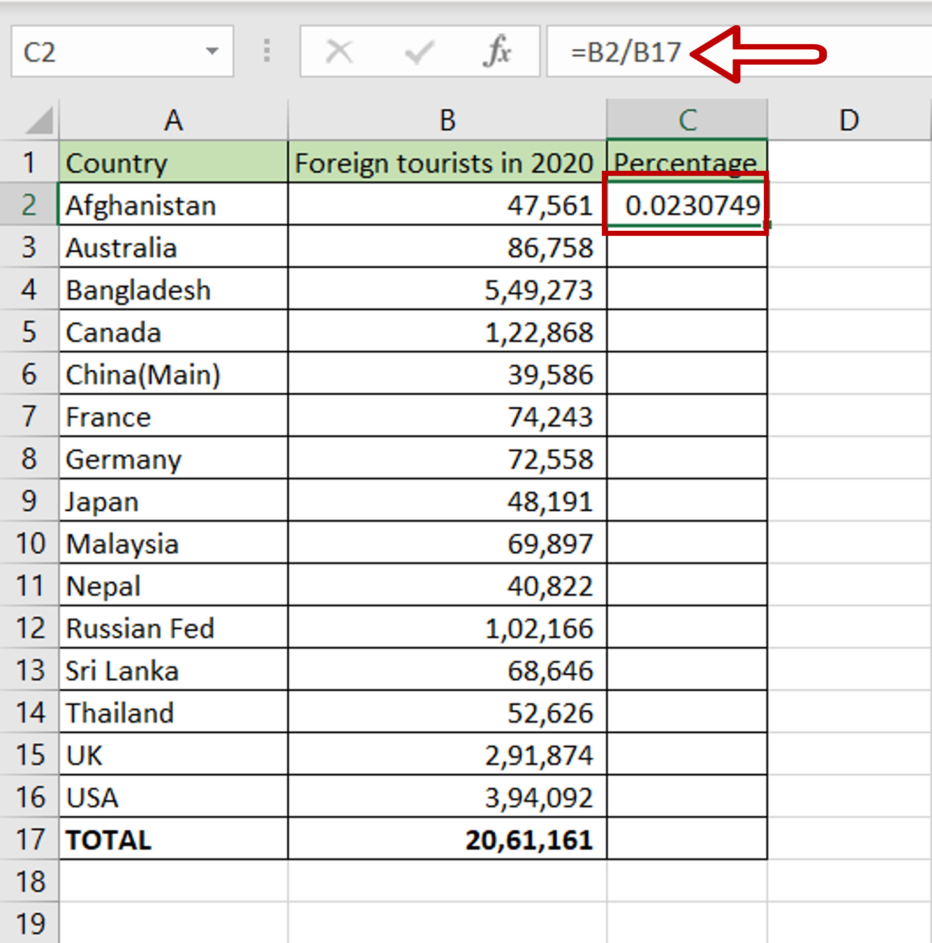
– In the first cell of the column in which the percentages are to be displayed, type the formula using cell references:
=( Foreign tourists in 2020/Total)
Step 2 – Make the ‘Total’ constant
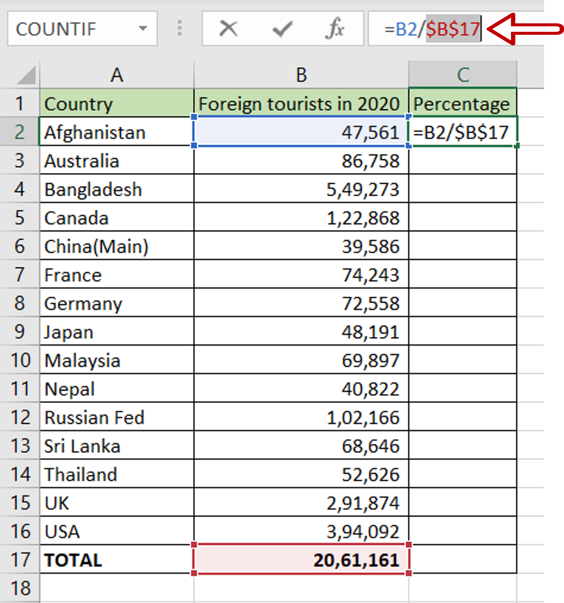
– Select cell reference for the ‘Total’ in the formula bar
– Press F4
– Dollar signs ($) are added to the cell reference to make it constant
Step 3 – Format the number as a percentage
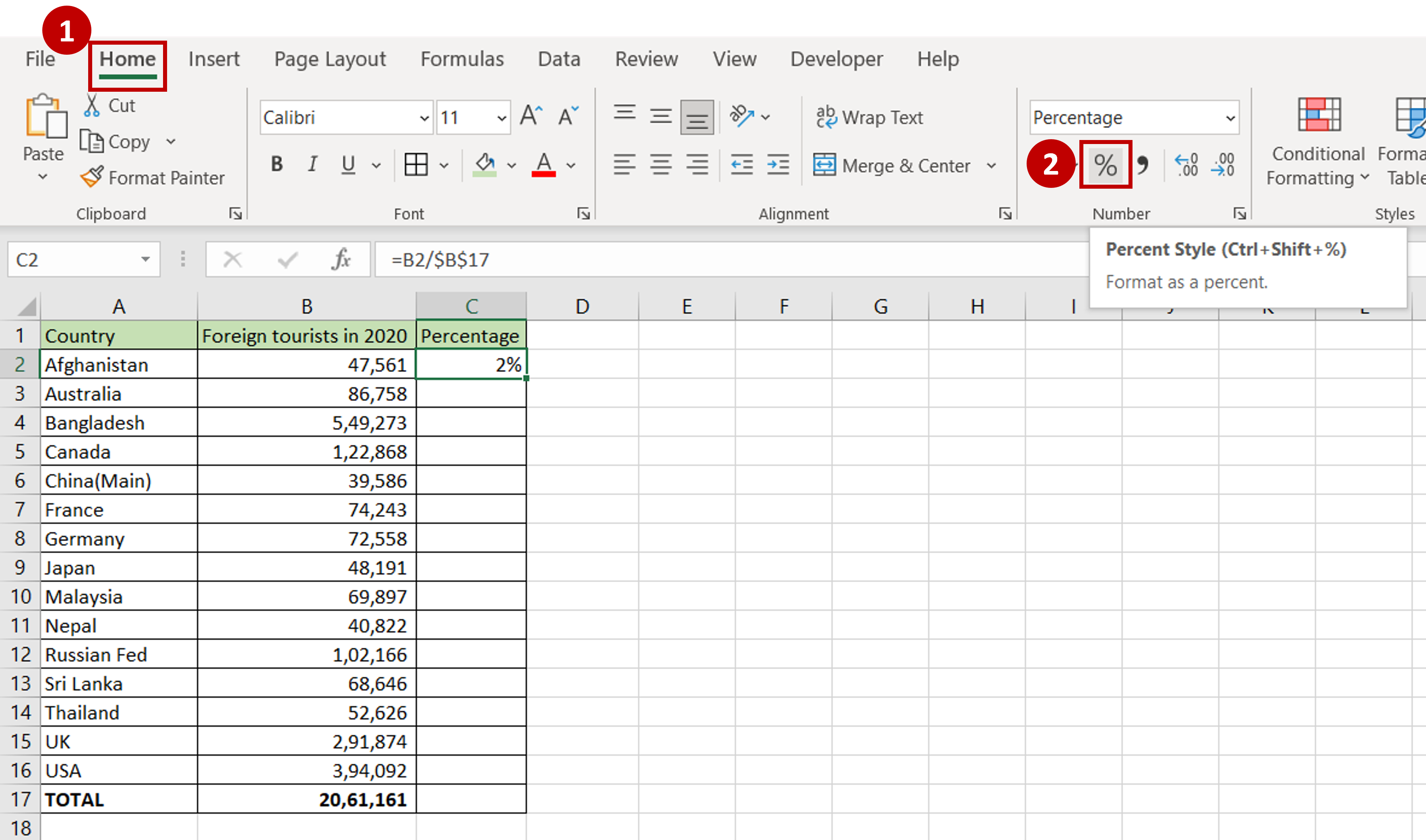
– Select the cell with the value
– Go to Home > Number
– Click on the percentage sign (%)
OR
Open the Format Cells window (Home > Number and click on the arrow to expand the menu OR Right-click and select Format Cells from the context menu OR Go to Home > Cells > Format > Format Cells) and select Number > Percentage and click OK
Step 4 – Copy the formula
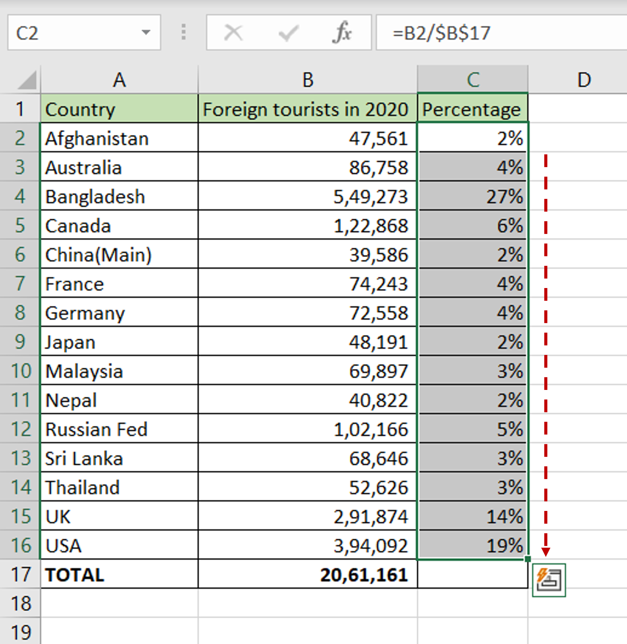
– Using the fill handle from the first cell, drag the formula to the remaining cells
OR
a) Select the cell with the formula and press Ctrl+C or choose Copy from the context menu (right-click)
b) Select the rest of the cells in the column and press Ctrl+V or choose Paste from the context menu (right-click)
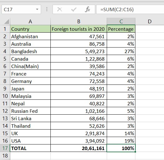
Step 5 – Sum the percentages
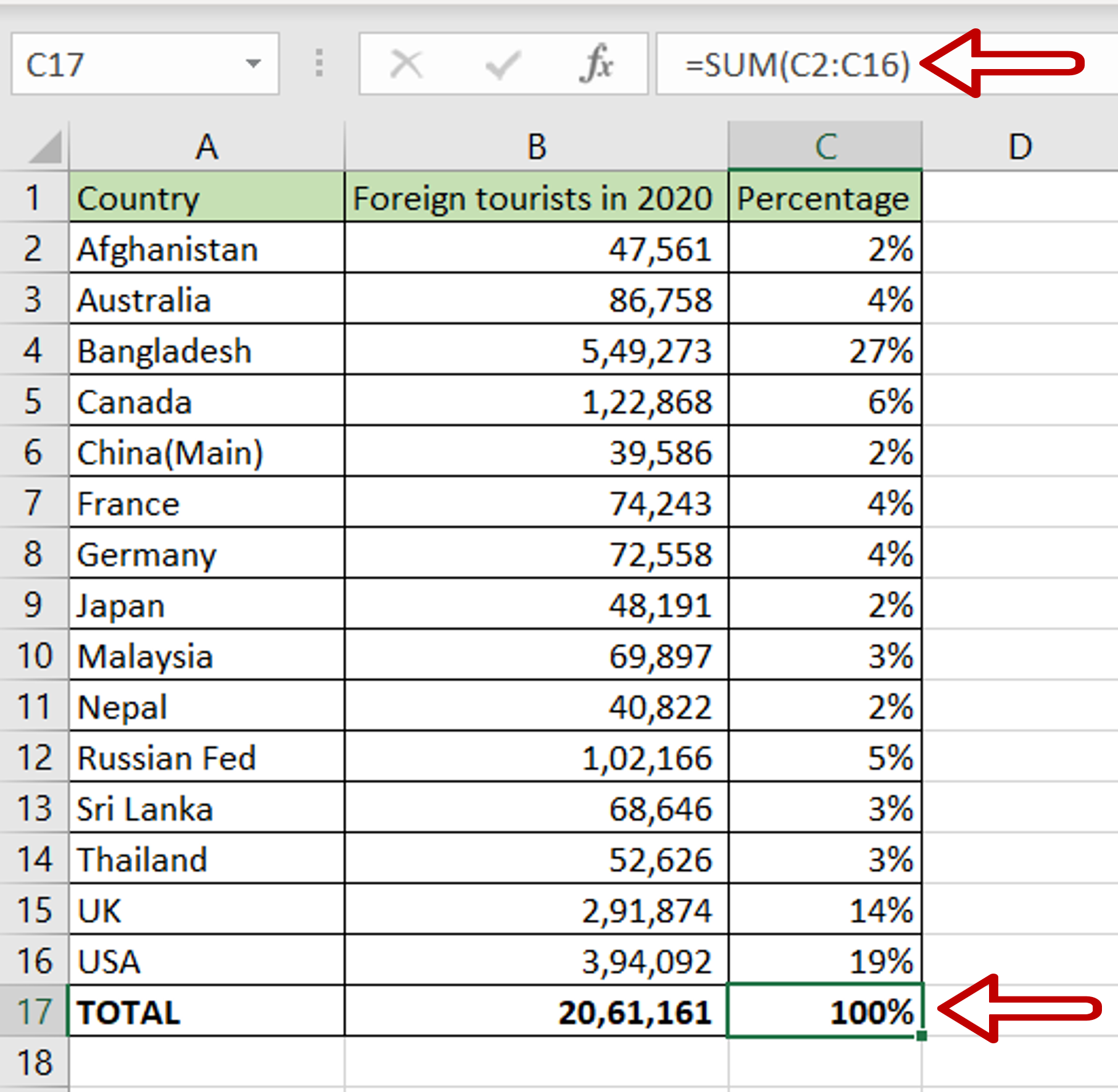
– Select the last cell of the column
– Type the formula using cell references:
=SUM(range of Percentages)
– Check that the total is 100%


