How to calculate the P value in Excel

You can watch a video tutorial here.

The P-value is used in hypothesis testing to help determine whether to accept or reject the null hypothesis. Excel is frequently used for such analysis. In Excel, we can compute the P-value using the Data Analysis tool or by using the T.TEST function. 

1. T.TEST() function: this is used to perform a Student’s T-test
2. Syntax: T.TEST (array1,array2,tails,type)
   1. array1: the range of the first data set
   2. array2: the range of the second data set.
   3. Tails: 1 for the one-tailed distribution and 2 for the two-tailed distribution.
   4. Type: the kind of T-Test to perform.

In this example, we look at the relationship between the kilometers driven and the selling price of previously-owned cars. 

Option 1 – Use the T.TEST() function

Step 1 – Create the formula

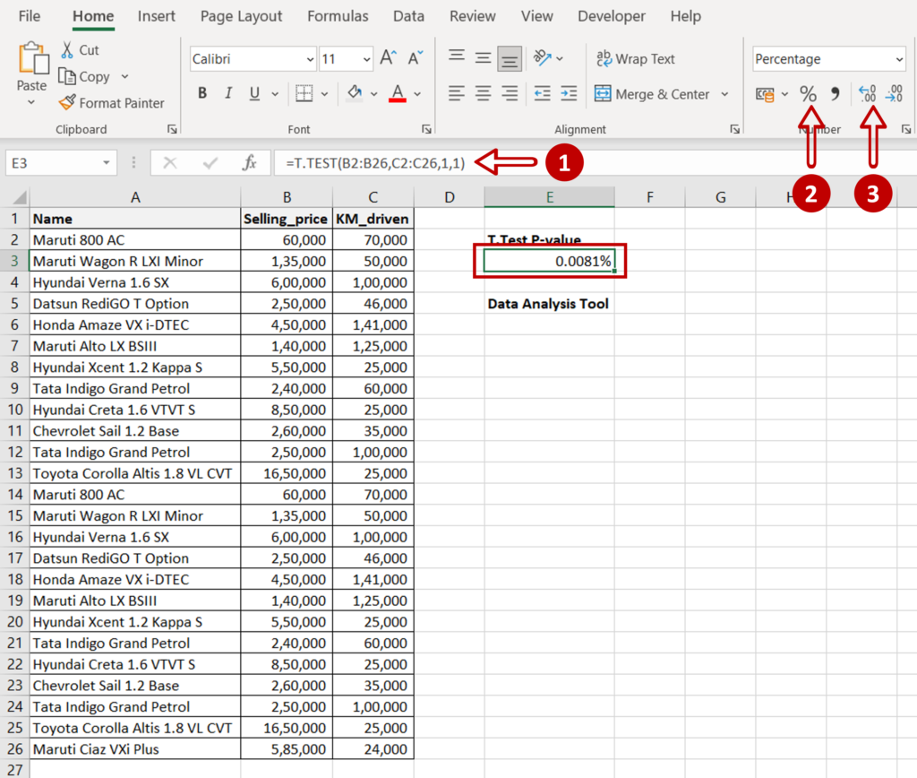
2. In the destination, type the formula, using cell references:

=T.TEST(range of Selling_Price, range of KM_driven,1,1)

3. Press Enter
4. The P-value is displayed
5. Format for percentage by clicking the Percent Style button (%) on the ribbon
6. Increase the decimal places by clicking the Increase decimal button on the ribbon

Options 2 – Use the Data Analysis tool

Note: If the Data Analysis button is present under Data > Analyze,  then skip steps 1 to 3

Step 1 – Open the Excel Options window

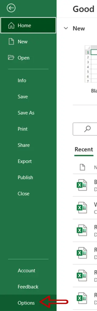
• Go to File > Options

Step 2 – Manage the Add-ins

7. Go to Add-ins
8. Select Excel Add-ins from the Manage drop-down
9. Click Go

Step 3 – Load the Analysis ToolPak add-in

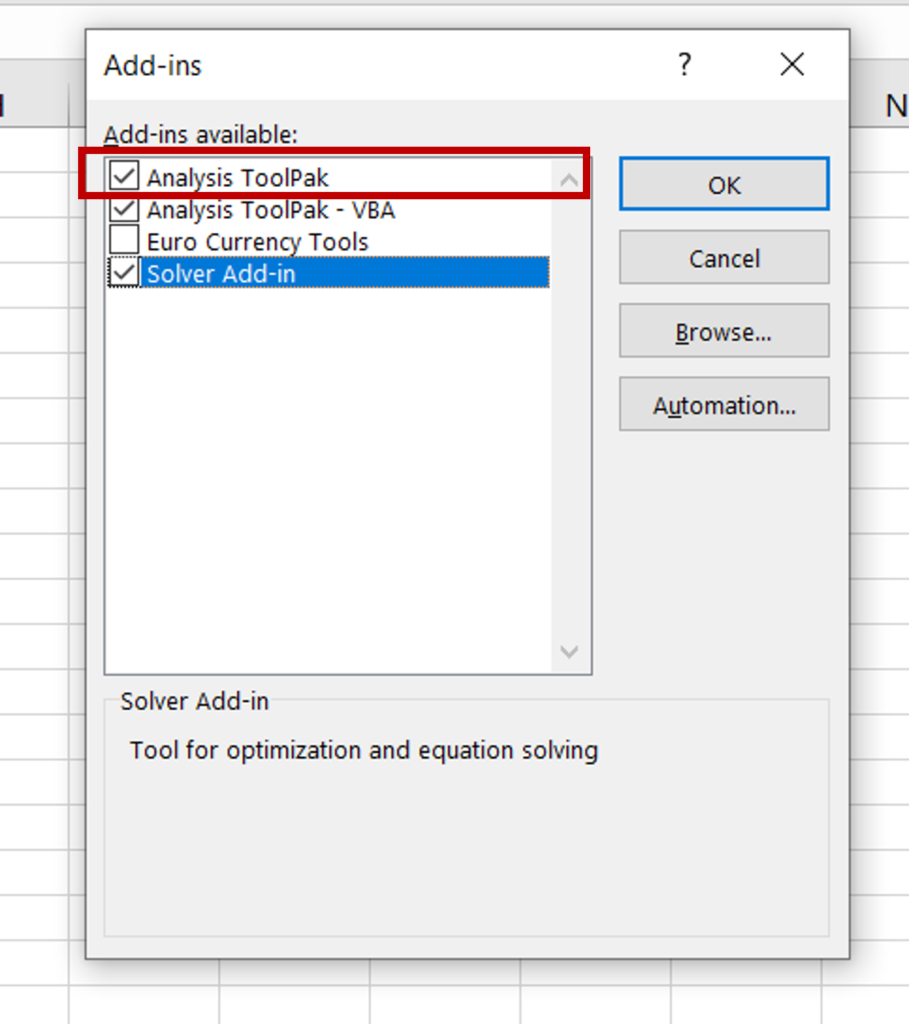
10. Select Analysis ToolPak
11. Click OK

Step 4 – Open the t-test: Paired Two Sample for Means window

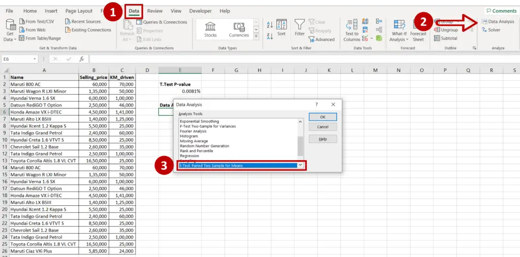
12. Go to Data > Analyze
13. Click on the Data Analysis button
14. In the window, select t-test: Paired Two Sample for Means
15. Click OK

Step 5 – Set the parameters

• Define the input ranges:
  • Input Y Range = the range of the first variable i.e. the ‘Selling Price’
  • Input X Range = and range of the second variable i.e. ‘KM_driven’ 
• Define the output range i.e where you want the result to be displayed
• Click OK

Step 6 – Check the result

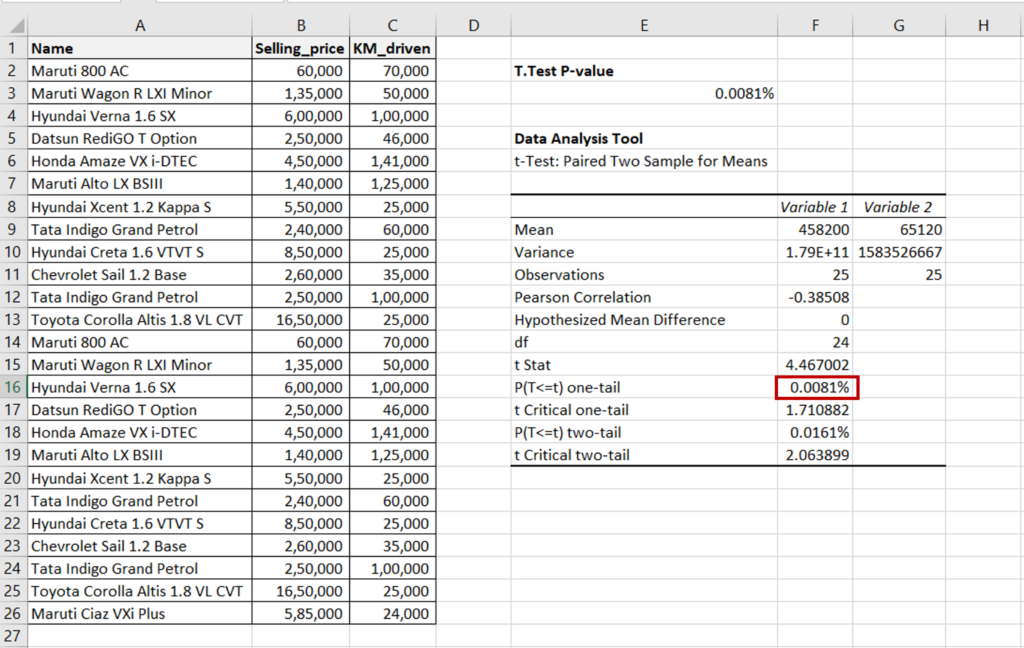
• The results of the test are displayed, including the P-value
• Format the P-value for percentage by clicking the Percent Style button (%) on the ribbon
• Increase the decimal places of the P-value by clicking the Increase decimal button on the ribbon