
How to calculate the last working day of the year in Excel
 By
SpreadCheaters
By
SpreadCheaters
In the given scenario, a company has employees with different job positions, and they receive salary increments on the last working day of the year, with varying dates based on their respective occupational roles. We will take this example to learn how to calculate the last working day of the year.
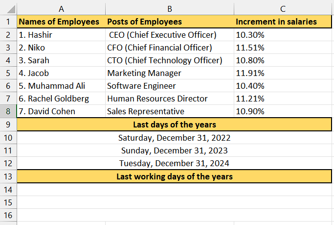
The last day of the year holds several important implications and significance across various contexts. We know that the last day of the year is the 31st of December but the last working day of every year is different and sometimes we need to calculate it for various purposes.
Step 1 – Selecting the cell
– Select any empty cell in which you want to calculate the last working day of the year.
– This particular cell will serve as the location to apply the aforementioned functions.
Step 2 – Writing the formula

– Begin by typing “WORKDAY” in the designated cell and then use the tab button on your keyboard to select the WORKDAY function.
– Proceed by entering “EOMONTH” in the same cell and use the tab button to select the EOMONTH function.
– Then select the cell which contains the last date of the year. For instance, it is A10 in our case.
– After that, write “0” (without quotes) as the second argument which indicates that we want the last day of the month of December for the specified date.
– Now, write “+1” (without quotes) which adds 1 to the result of the EOMONTH function, effectively moving to the first day of the next month.
– Our formula applies the WORKDAY function to the adjusted date from the above step.
“EOMONTH(A10,0)+1” provides the start date for the WORKDAY function, which is the first day of the following month.
– After that, write “-1” as the second argument which specifies that we want to subtract one working day from the start date to get the last working day of the month of December which is actually the last month of the year so, it will give us the last working day of the year.
– Eventually, our formula would look like this,
=WORKDAY(EOMONTH(A10,0)+1,-1
Step 3 – Implementing the formula
– After you’ve followed the above steps, add the closing parenthesis.
– Then, press Enter button and the last working day of the year would appear. For instance, the last working day of 2022 appears which is Friday, December 29, 2022, whereas the last day of the year was on Saturday which is considered a holiday.
Step 4 – Implementing formula for all last days of years given
– For applying the formula on the whole range, select the cell in which the result is present. For example, it is an A10 cell in our case.
– Then, position your cursor on the bottom-right corner of the cell until it transforms into a plus (+) shape, known as the fill handle.
– Lastly, by dragging down the fill handle to the desired cells, you can apply the formula to those cells as well. The formula will be automatically extended to the selected range, ensuring consistent application throughout.


