How to calculate the beta of a stock in Excel
 By
SpreadCheaters
By
SpreadCheaters
In investing, it is important to know the beta of a stock. It helps the investor to measure the volatility of the stock’s risk. It indicates how much a stock’s price fluctuates up and down in relation to other equities in the stock market. Luckily, Excel can let you calculate this in two easy ways:
- Using functions COVARIANCE.P and VAR.P
- Using SLOPE Function
Let us learn these three Excel Statistical Functions before diving into the tutorial.
COVARIANCE.P
COVARIANCE.P function is used to determine the relationship between the two sets of data. The syntax of the function is written as below:
=COVARIANCE.P(array1,array2)
The arguments are the two data sets that you wish to get the covariance. Both are arrays of cells that contain integer values. But you must remember that both of the arrays must have an equal number of data points or else you will get an error as a result.
VAR.P
VAR.P function returns the variance of the entire population. It is different from VAR.S which only returns the variance of a sample of a population. The arguments of the function syntax is as below:
=VAR.P(number1,[number2],..)
The first argument is required and it corresponds to a population, while the second argument is optional and also corresponds to a population..
SLOPE
=SLOPE(known_y’s,known_x’s)
Lastly, SLOPE function returns the slope of the linear regression line through its arguments: known_y’s and known_x’s. Both arguments are required and both are a set of data points.
Now that we are familiar with the three functions, let us now learn the steps on calculating the beta of a stock. Please take note that both of the methods have the same first three steps.
Step 1 – Obtain the historical security prices.
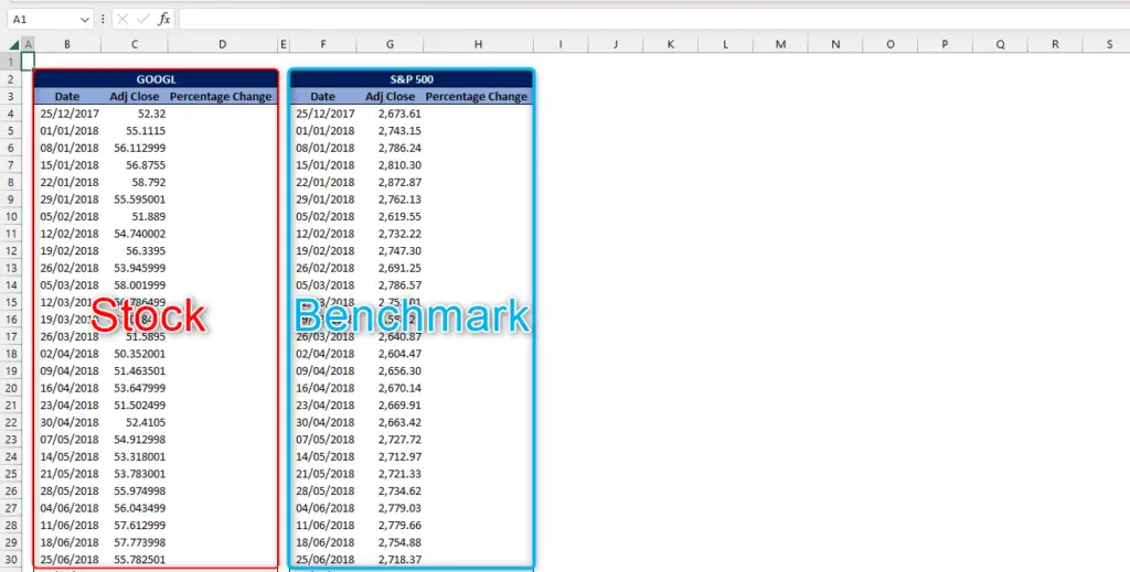
- Obtain the historical security prices of the stock that you want to measure
- Obtain the historical security prices of the benchmark (S&P 500)
- Combine both data in a spreadsheet. The datapoints that we will be needing is their adjusted closing price.
Step 2 – Determining Percentage Change of the Stock
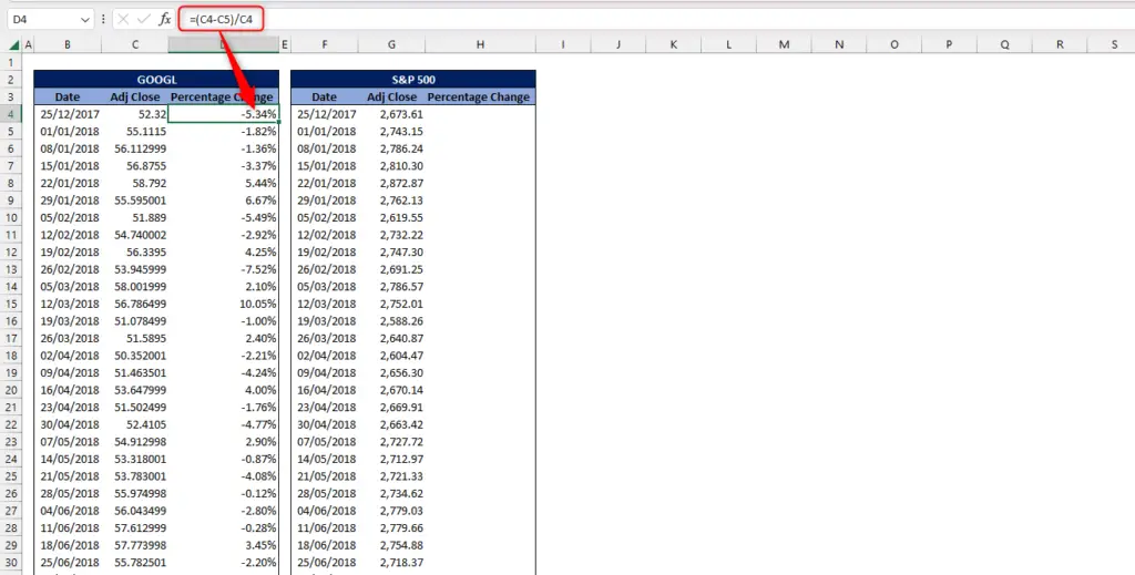
- The formula of percentage change is old value minus new value all over old value
=(C4-C5)/C4
- Change the number format to percentage
- Extend the formula down to the bottom of the list
Step 3 – Determining Percentage Change of the benchmark
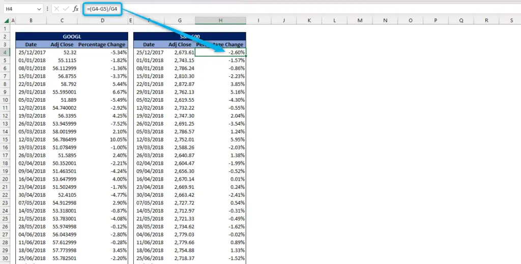
- Same with Step 2, the formula of the percentage change is old value minus new value all over old value
=(G4-G5)/G4
- Change the number format to percentage
- Extend the formula down to the bottom of the list
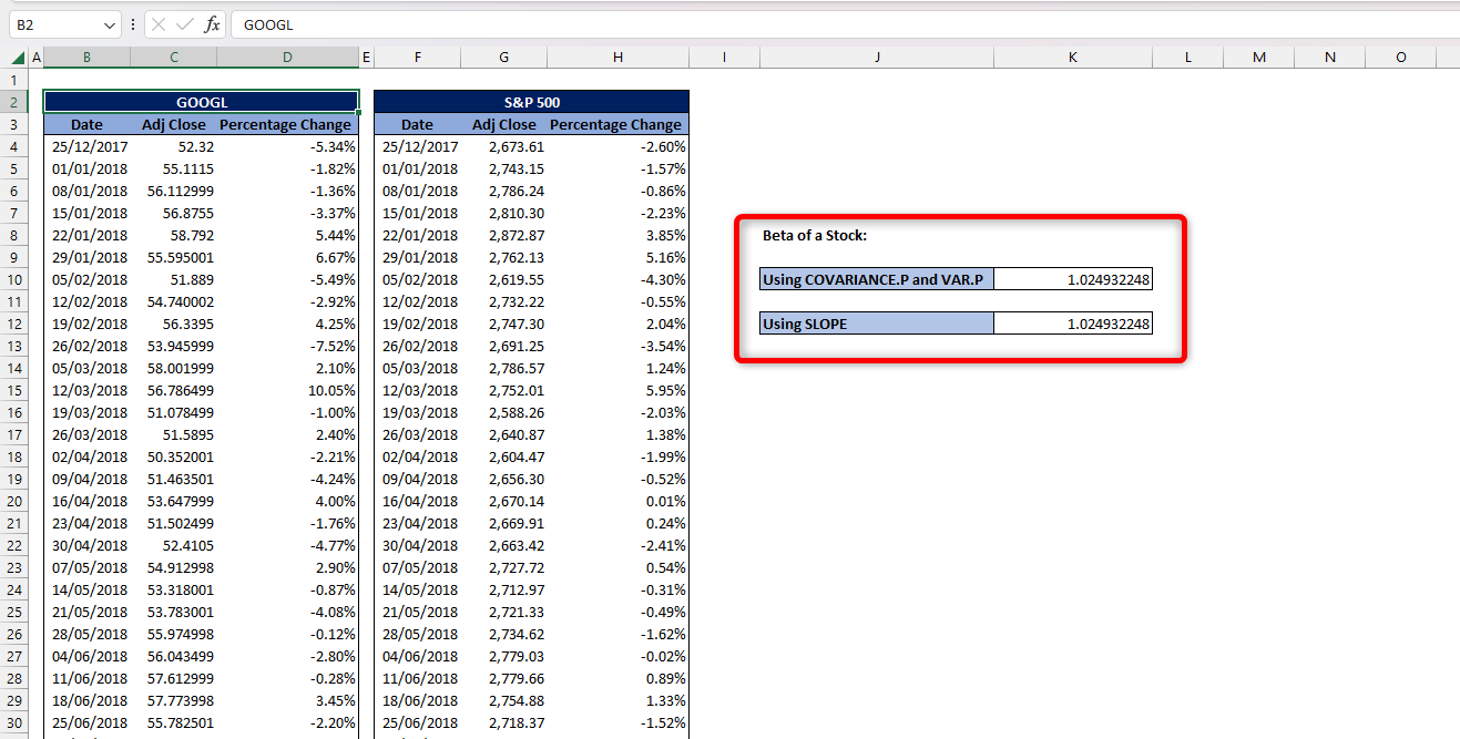
Step 4 – Getting the Beta of a stock
Method 1: Using COVARIANCE.P and VAR.P
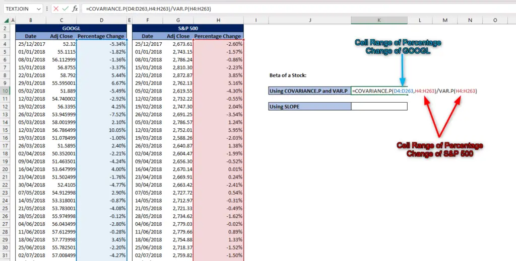
=COVARIANCE.P(array1,array2)/VAR.P(number1,[number2],..)
- For the COVARIANCE.P function, array1 is the cell range that contains the percentage change of the stock while array 2 is the cell range that contains the percentage change of the benchmark.
- And then for the VAR.P function, use the cell range that contains the percentage change of the benchmark.
=COVARIANCE.P(D4:D263,H4:H263)/VAR.P(H4:H263)
Method 2: Using SLOPE function
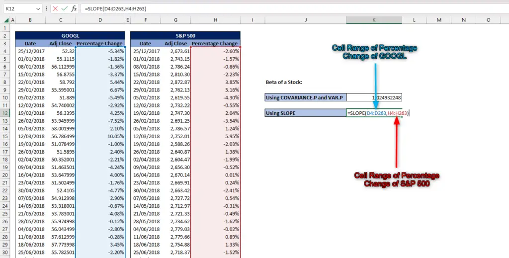
- The use of SLOPE function is straightforward.
- Argument known_y’s is the array of cell that contains the percentage change of the stock
- While argument known_x’s is the array of cell that contains the percentage change of the benchmark
=SLOPE(D4:D263,H4:H263)
Both of these methods will result in the same number. Change its number format to ‘General’ if it automatically changes to ‘Percentage’. In financial analysis, the result of 1.024932248 denotes that the stock is more volatile than the market.