
How to calculate tenure in years and months in Microsoft Excel
 By
SpreadCheaters
By
SpreadCheaters
Calculating tenure in years and months in Excel involves determining the length of time that an individual has been employed in a company or organization, expressed in both years and months. Calculating tenure in years and months in Excel can help organizations track employee performance, make informed decisions about promotions and salary increases, and identify areas where additional training or support may be needed.
In this tutorial, we will learn how to calculate tenure in years and months in Microsoft Excel. In Microsoft Excel calculating tenure in years and months is a simple process. We can utilize various built-in functions for this i.e. YEARFRAC, YEAR, and DATEDIF. We can also calculate the tenure in years using simple algebraic calculations.
We possess a dataset that indicates the starting and ending dates of employment of certain workers in a firm. Our objective is to determine their tenure of service both in years and months.
Method 1: Using the DATEDIF Function to Calculate Tenure
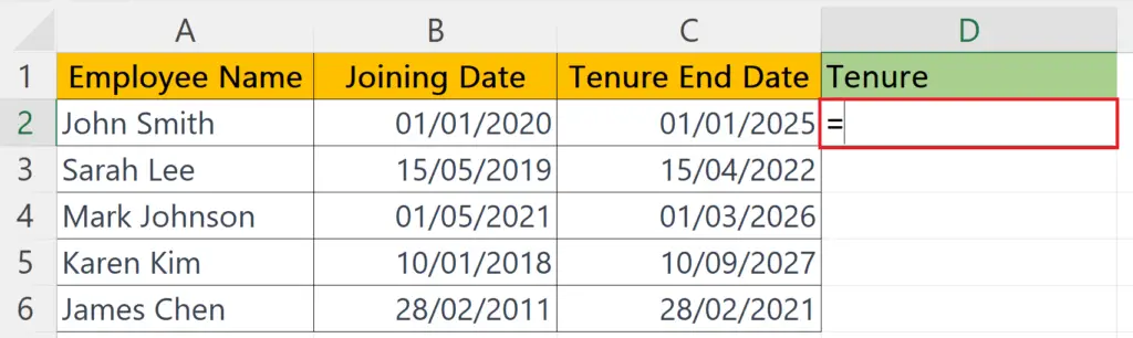
Step 1 – Select a Blank Cell and Place an Equals Sign
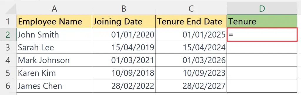
- Select a blank cell where you want to calculate the tenure.
- Place an Equals sign.
Step 2 – Use the DATEDIF Function to Calculate the Years
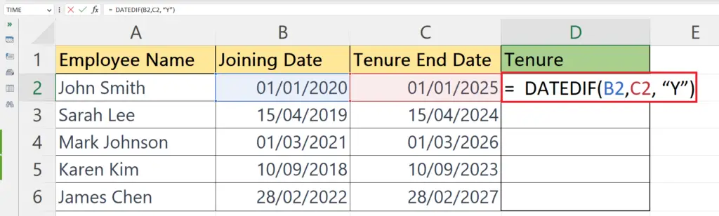
- The DATEDIF function is commonly used to extract years, months, or even days in Excel.
- The syntax to calculate months of the tenure will be:
DATEDIF(B2,C2, “Y”)
- Where C2 and B2 are the end date and start date, respectively.
- The third argument “Y” specifies the information to be extracted i.e. years.
Step 3 – Enter an Ampersand Operator and Enter “Year”
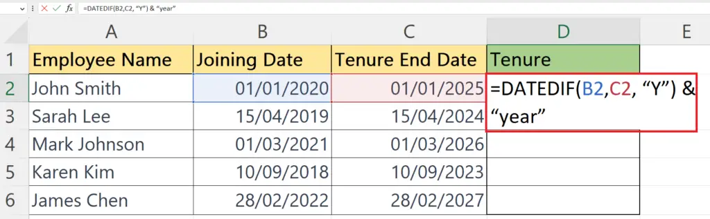
- Enter an Ampersand operator next to the DATEDIF function.
- Then, enter “years” as we are extracting years from the first DATEDIF function.
- The syntax will be:
DATEDIF(B2,C2, “Y”) & “year”
Step 4 – Use the DATEDIF Function to Calculate the Months
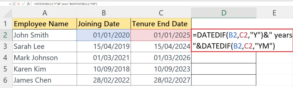
- The syntax to calculate months of the tenure will be:
DATEDIF(B2,C2, “Y”) & “year” & DATEDIF(B2,C2, “YM”)
- Where C2 and B2 are the end date and start date, respectively.
- The third argument “YM” specifies the information to be extracted i.e. months.
Step 5 – Enter an Ampersand Operator and Enter “Month”
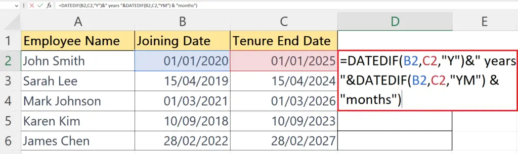
- Enter an Ampersand operator next to the DATEDIF function.
- Then, enter “months” as we are extracting months from the second DATEDIF function.
DATEDIF(B2,C2, “Y”) & “year” & DATEDIF(B2,C2, “YM”) & “months”
Step 6 – Press the Enter Key
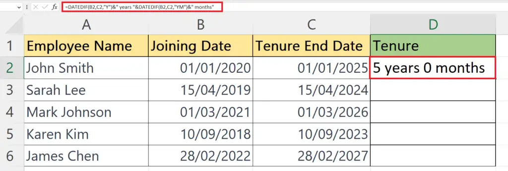
- Press the Enter key.
Step 7 – Use Autofill to Calculate the Tenure for Each Employee
- Use Autofill to calculate the tenure for each employee.
Method 2: Using the YEARFRAC Function to Calculate the Tenure
Step 1 – Select a Blank Cell and Place an Equals Sign
- Select a blank cell.
- Place an equals sign.
Step 2 – Enter the First YEARFRAC Function to Extract Years
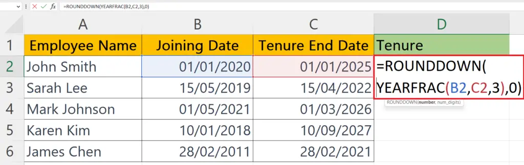
- The syntax would be:
ROUND(YEARFRAC(B2,C2,3),0)
- The first argument of the YEARFRAC function i.e. B2 is the start date and the second argument i.e. C2 is the end date.
Step 3 – Enter an Ampersand and Enter “ years “
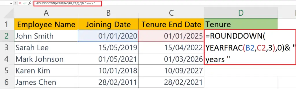
- Enter an ampersand operator next to the YEARFRAC function.
- Enter “ years “ next to the ampersand operator.
ROUND(YEARFRAC(B2,C2,3),0)&” years ”
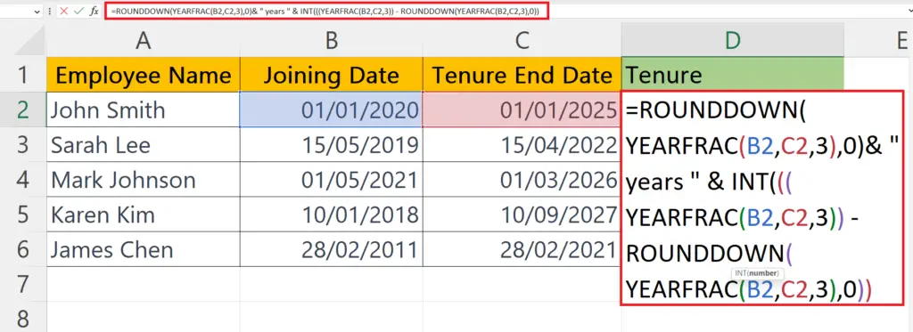
Step 4 – Enter the INT Function and the Second YEARFRAC Function to get the Months
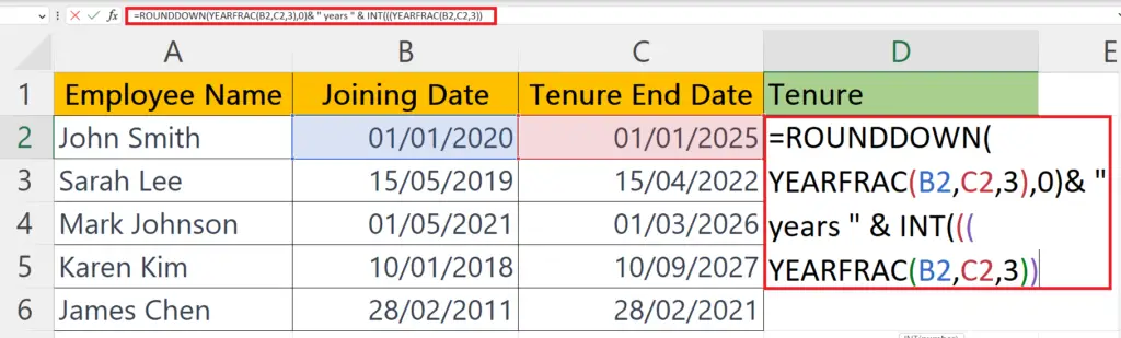
- Enter the INT function.
- Nest the second YEARFRAC function inside the INT function.
- Open three parentheses before the second YEARFRAC function.
- The syntax would become:
ROUND(YEARFRAC(B2,C2,3),0)&” years ” & INT(((YEARFRAC(B2,C2,3))
Step 5 – Now Place a Subtraction Sign
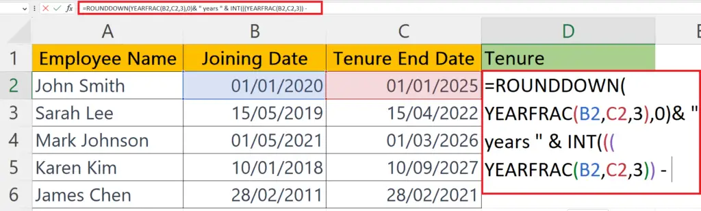
- Now place a subtraction sign.
Step 6 – Enter ROUNDDOWN Function and Enter the Third YEARFRAC Function as ROUNDDOWN’S First Argument
- Enter ROUNDDOWN Function.
- Enter the third YEARFRAC function.
| ROUND(YEARFRAC(B2,C2,3),0)&”year”&INT(((YEARFRAC(B2,C2,3))-ROUNDDOWN(YEARFRAC(B2,C2,3),0)) |
Step 7 – Multiple by 12 and Close a Parenthesis
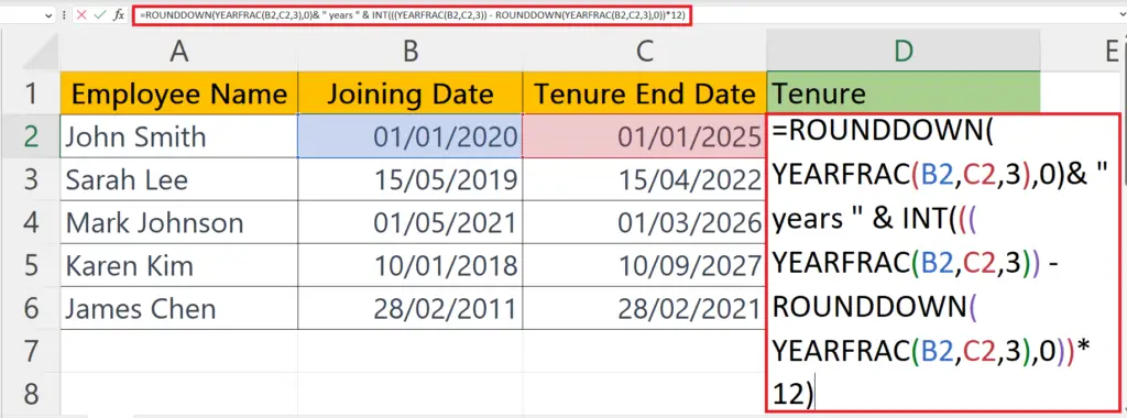
- Multiple by 12 and close parentheses.
| ROUND(YEARFRAC(B2,C2,3),0)&”years”&INT(((YEARFRAC(B2,C2,3))-ROUNDDOWN(YEARFRAC(B2,C2,3),0))*12 ) |
Step 8 – Enter an Ampersand and Enter “ months”
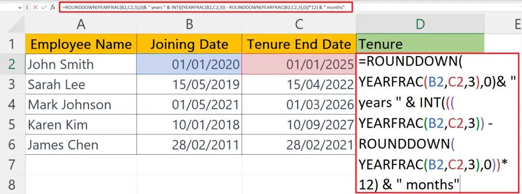
- Enter an Ampersand operator and enter “Months”.
| ROUND(YEARFRAC(B2,C2,3),0)&”years”&INT(((YEARFRAC(B2,C2,3))-ROUNDDOWN(YEARFRAC(B2,C2,3),0))*12 ) & ” months” |
Step 9 – Press the Enter Key
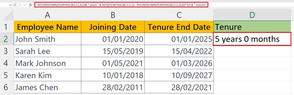
- Press the Enter key.
Step 10 – Use Autofill to Apply the Formulae on Each Cell
- Use Autofill to apply the formulae on each cell.
Breakdown of the Formulae:
ROUND(YEARFRAC(B2,C2,3),0)&”years”&INT(((YEARFRAC(B2,C2,3))-ROUNDDOWN(YEARFRAC(B2,C2,3),0))*12 ) & ” months”
- YEARFRAC(B2,C2,3) calculates the fraction of a year between two dates in cells B2 and C2 using the “actual/actual” method (denoted by the number 3).
- ROUND(YEARFRAC(B2,C2,3),0) rounds this fraction to the nearest whole number of years.
- “years” is a string of text that is added to the result from step 2 to indicate the unit of measurement.
- ROUNDDOWN(YEARFRAC(B2,C2,3),0) rounds the fraction of a year down to the nearest whole number of years.
- (YEARFRAC(B2,C2,3))-ROUNDDOWN(YEARFRAC(B2,C2,3),0) calculates the fraction of a year that is left over after step 4.
- ((YEARFRAC(B2,C2,3))-ROUNDDOWN(YEARFRAC(B2,C2,3),0))*12 multiplies the fraction of a year from step 5 by 12 to convert it to months.
- INT(((YEARFRAC(B2,C2,3))-ROUNDDOWN(YEARFRAC(B2,C2,3),0))*12) rounds the number of months down to the nearest whole number.
- ” months” is a string of text that is added to the result from step 7 to indicate the unit of measurement.
- The & symbol is used to concatenate the results from steps 3 and 8 with the result from step 2, resulting in a single string that reads “X years Y months”.


