
How to calculate sum if cell contains a specific text using SUMIF in Excel
 By
SpreadCheaters
By
SpreadCheaters
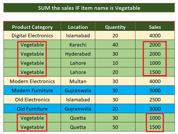
In today’s tutorial we’ll learn how to calculate the sum of cells based on a text criterion in Excel. Let’s take a look at the following sales dataset.
To use the SUMIF formula let’s first understand the syntax of the formula. The generic formula can be written as follow;
=SUMIF(range,”*text*”,sum_range)
The SUMIF function syntax has the following arguments:
- range Required Parameter.
The range of cells that you want evaluated by criteria. Cells in each range must be numbers or names, arrays, or references that contain numbers. Blank and text values are ignored. The selected range may contain dates in standard Excel format (examples below).
- criteria Required Parameter.
The criteria in the form of a number, expression, a cell reference, text, or a function that defines which cells will be added. Wildcard characters can be included – a question mark (?) to match any single character, an asterisk (*) to match any sequence of characters. If you want to find an actual question mark or asterisk, type a tilde (~) preceding the character. For example, criteria can be expressed as 32, “>32”, B5, “3?”, “apple*”, “*~?”, or TODAY().
Important: Any text criteria or any criteria that includes logical or mathematical symbols must be enclosed in double quotation marks (“). If the criteria is numeric, double quotation marks are not required.
- sum_range Optional.
The actual cells to add, if you want to add cells other than those specified in the range argument. If the sum_range argument is omitted, Excel adds the cells that are specified in the range argument (the same cells to which the criteria is applied).Sum_range should be the same size and shape as range. If it isn’t, performance may suffer, and the formula will sum a range of cells that starts with the first cell in sum_range but has the same dimension as range.
- For example:
| range | sum_range | Actual summed cells |
|---|---|---|
| A5:A10 | B5:B10 | B5:B10 |
| A11:A20 | B11:K5 | B11:B20 |
Let’s assume that we wish to find the sum of the sales for Vegetables only then we can use SUMIF with “Vegetable” as text criteria, Product Category as range and Sales column as the sum_range.
Sometimes your data in Excel spreadsheets contains special text tags or names to identify them from other data and we are asked to calculate the sum of the cells related to that specific text tag. In this case Microsoft Excel provide us with a simple method to do the same.
Step 1 – Create an appropriate formula using SUMIF
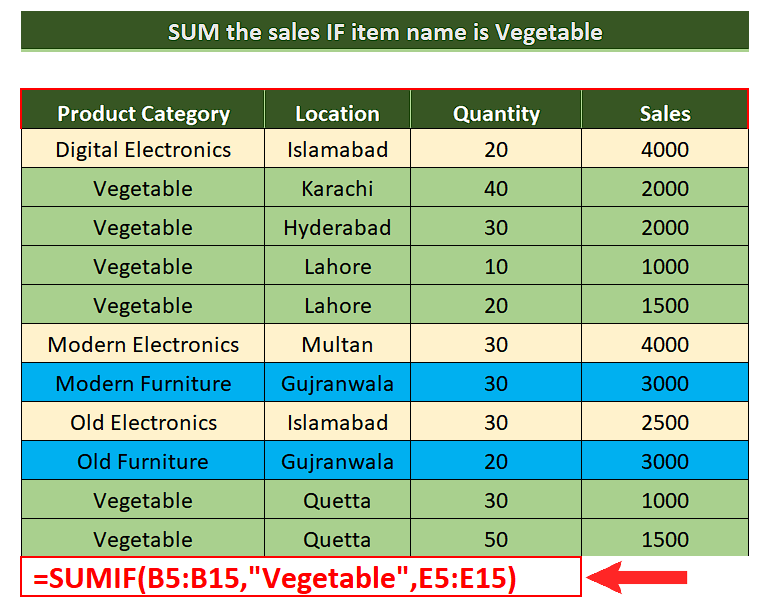
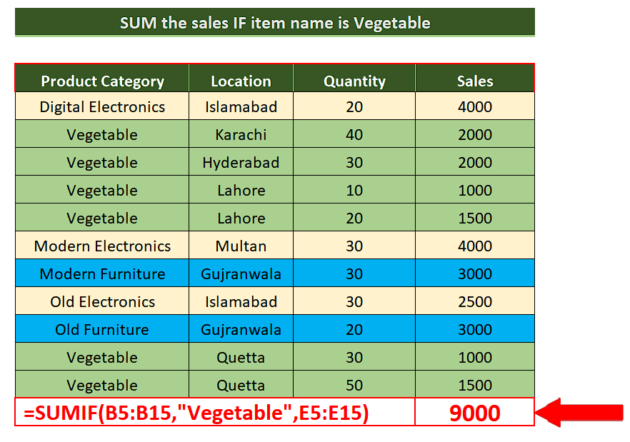
– We wish to calculate the sales of vegetables so we’ll use the following formula in a suitable cell;
=SUMIF(B5:B15,”Vegetable”,E5:E15)
Step 2 – Implement the formula
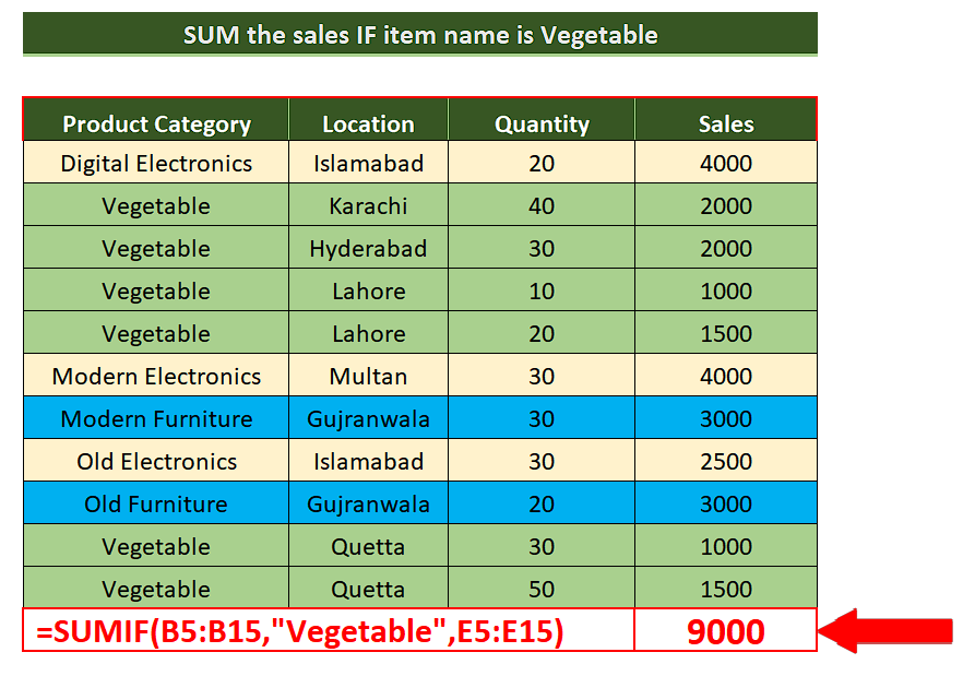
– Now that we have created our desired formula, we will press enter and the formula will be implemented in the suitable cell as shown above.


