
How to calculate stem and leaf plot in Excel
 By
SpreadCheaters
By
SpreadCheaters
Let’s have a series of two digit numbers in our data set as shown.
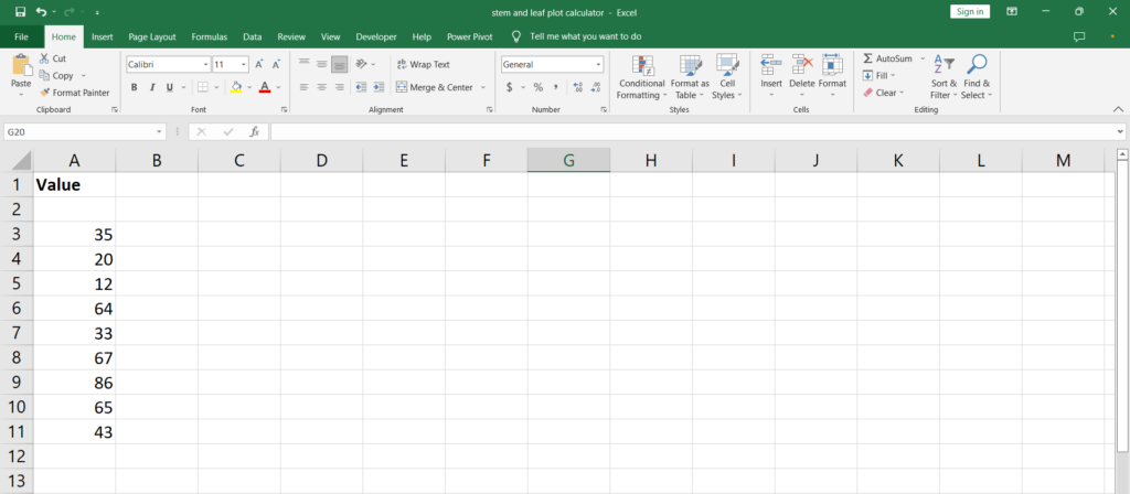
A stem and leaf plot is a great statistical tool to identify the central tendency, spread, maximum and minimum value in a continuous data set. Let’s see how we can create a stem and leaf plot calculator in excel.
Step 1 – Identifying stems and leaves
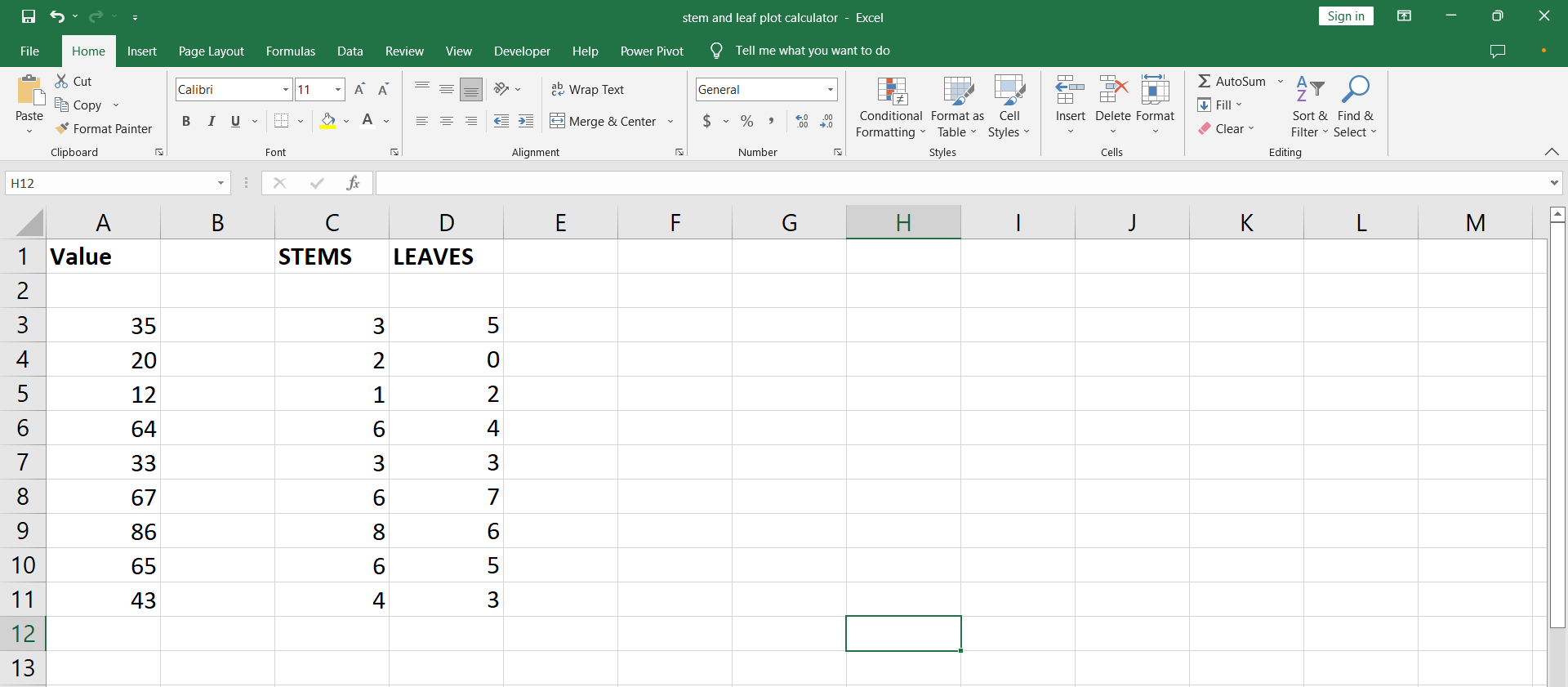
– The first step is to identify the stems and write them in a new column called Stems. Next to the cell containing Stems type the text Leaves.
– In a given number the stem is all the digits except the last one. So in the case of 43, 4 is the stem and 3 is the leaf.
– Similarly if the number is in hundreds such as 128, the stem is 12 and leaf is 8.
Step 2 – Understanding functions
– To calculate the leaves we are going to use two excel functions here. One is the REPT function and the other is the COUNTIF function.
– The syntax for both the REPT and COUNTIF is given below.
REPT(text, number_times)
COUNTIF(range, criteria)
– The REPT function is used to repeat a text a given number of times.
– The COUNTIF function counts a value in a given range based on a specific criteria and outputs the evaluated count.
Step 3 – Implement the formula

– Now we are going to implement the formula in the excel worksheet shown before.
– Write the stems from in the column. If we have a smaller set of numbers this can be done manually.
– However, if the set is large just write the 1 in a cell and then 2 in the cell below it. Select the two cells and use the fill handle i.e. the small green cross at the bottom right of the selected cell set, to drag down up to whichever digit you want the series to end up at.
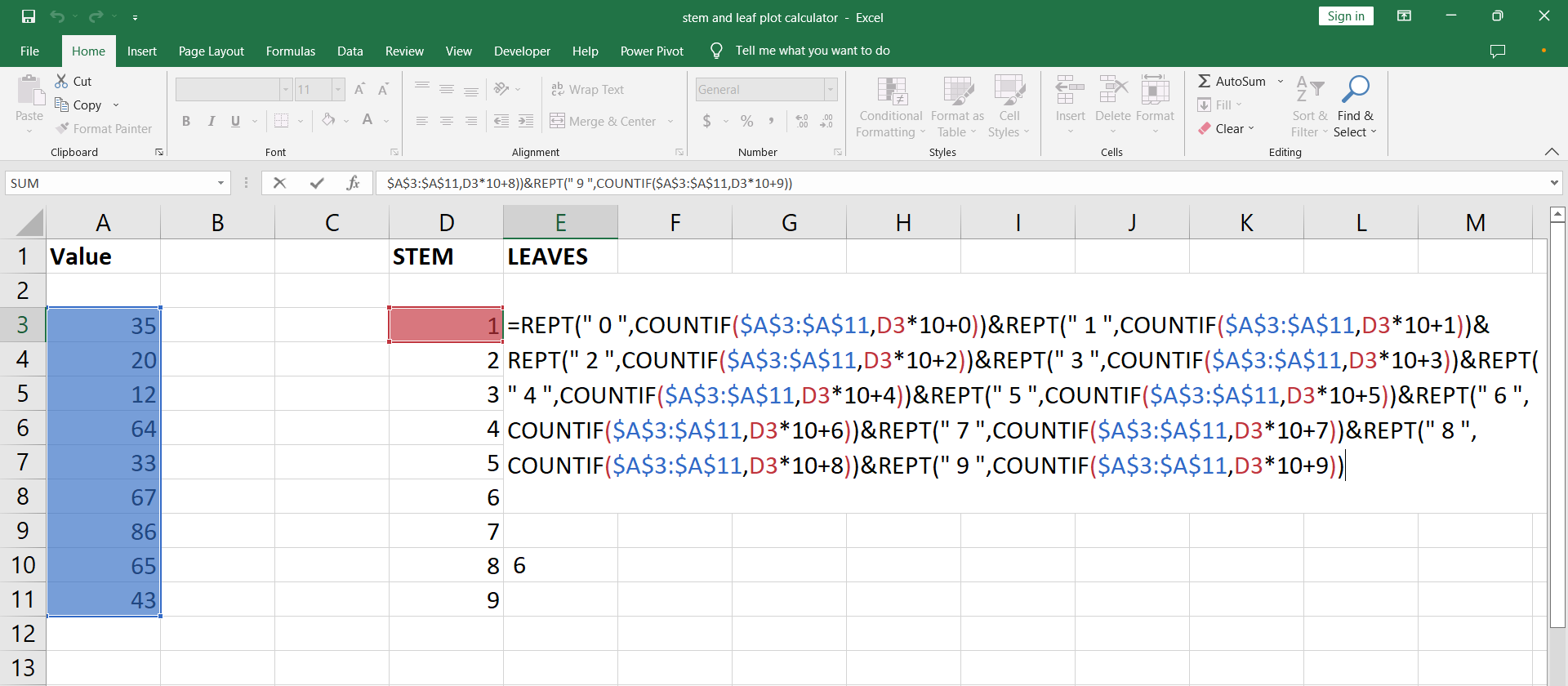
– So now that we have created stems. We can start writing the formula. Click the cell next to the 1 in the stems column and write the formula as follows,
=REPT(” 0 “, COUNTIF($A$3:$A$11,D3*10+0))
– The above formula will count the required number in the range of numbers A3 to A11. D3 in our case contains 1 so the number to find in the given range is 1 times 10 plus 0 which evaluates to 10. So the required number is 10. However many times 10 is counted the text “ 0 ” will be repeated in the E3.
– Next we are going to repeat the formula in the same cell E3 with an ampersand & written in between but every time the text will contain the next digit. i.e. “ 1 ” for the text in the next formula, “ 2 ” in the next and so on.
=REPT(” 0 “,COUNTIF($A$3:$A$11,D3*10+0))&REPT(” 1 “,COUNTIF($A$3:$A$11,D3*10+1))&REPT(” 2 “,COUNTIF($A$3:$A$11,D3*10+2))&REPT(” 3 “,COUNTIF($A$3:$A$11,D3*10+3))&REPT(” 4 “,COUNTIF($A$3:$A$11,D3*10+4))&REPT(” 5 “,COUNTIF($A$3:$A$11,D3*10+5))&REPT(” 6 “,COUNTIF($A$3:$A$11,D3*10+6))&REPT(” 7 “,COUNTIF($A$3:$A$11,D3*10+7))&REPT(” 8 “,COUNTIF($A$3:$A$11,D3*10+8))&REPT(” 9 “,COUNTIF($A$3:$A$11,D3*10+9))
– Copy the above formula and paste in the formula bar for cell D3.This looks lengthy but we have to write it only once and then use the fill handle to fill the rest of the cells in the column of Leaves.
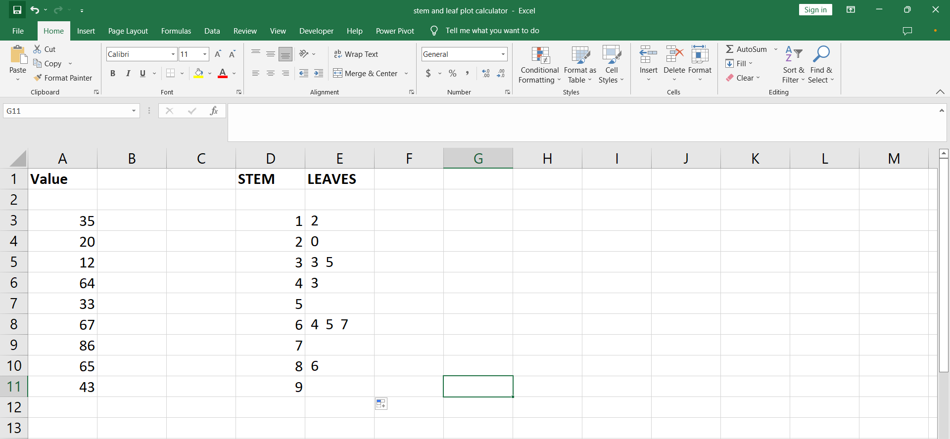
– Use the fill handle by dragging or double clicking to implement the formula for the cells above. The final result is shown in the image above.


