
How To Calculate Sharpe Ratio In MS Excel
 By
SpreadCheaters
By
SpreadCheaters
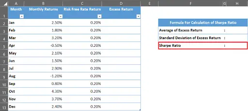
Also known as Sharpe Index, it is used to calculate the performance of an investment considering all the related risks. It compares investments of different risk profiles against each other. Let’s understand how it can be calculated in MS Excel with the following example:
We have investment data & want to find out the sharpe ratio for the investment.
Note: All the data in the above table is formatted as Percentage with 2 decimal places through cell formatting options.

The Sharpe Ratio is a commonly used benchmark that describes how well an investment uses risk to get return. Given several investment choices, the Sharpe Ratio can be used to quickly decide which one is a better use of your money.
Step 1 – Calculate Value of Excess Return
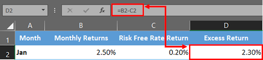
– First we need to find out the value of Excess Return.
– This can be calculated by subtracting Monthly Returns with Risk Free Rate Return.
Step 2 – Drag The Formula Down Below
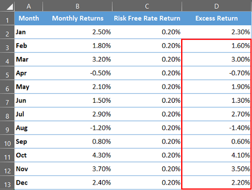
– With the help of a selection handle, drag the formula to the remaining cells.
Step 3 – Calculate Average of Excess Return
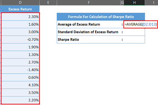
– Now find out the average of Excess Return using below formula & press enter.
Step 4 – Calculate Standard Deviation of Excess Return
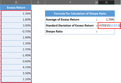
– Next we will find out the standard deviation of Excess Return using below formula & press enter.
Step 5 – Find Out The Sharpe Ratio
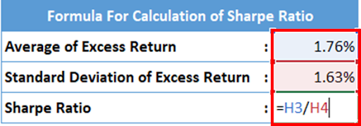
– Let’s find out the sharpe ratio by dividing Average of Excess Return with Standard Deviation of Excess Return.
Step 6 – Calculation of Sharpe Ratio
– Sharpe ratio can be calculated through these simple steps.


