How to calculate percentage in pivot table
In this tutorial we will learn how to calculate the percentage in the pivot table. This dataset includes three columns: “Region,” “Product,” “Profit ”and “Sales.” Each row represents a different sale, with the corresponding region, product, and sales amount. Major steps to calculate percentage in pivot table are given below.
A pivot table is a powerful feature in Excel that allows users to summarize and analyze large datasets by grouping and aggregating data based on various criteria, such as categories or variables. Pivot table percentage is a calculation option within a pivot table that provides the percentage of a specific value or subtotal in relation to the total value or subtotal, offering valuable insights into the data distribution.
Step 1 – Make pivot table

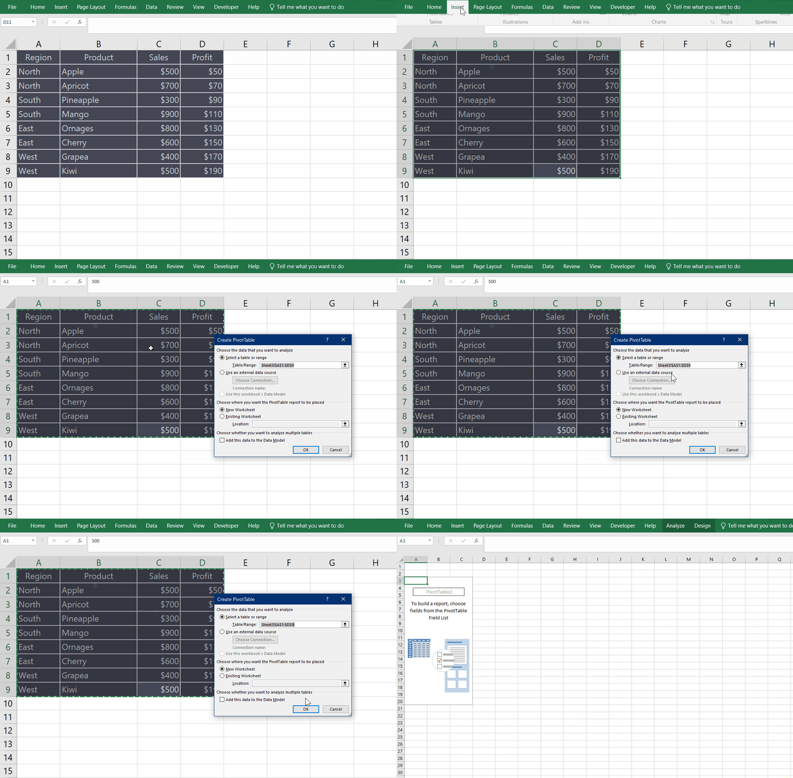
– Open the spreadsheet.
– Select the data range.
– Click on the Insert menu.
– Click on the first icon Pivot table.
– A dialogue box will open.
– The data range will be shown and the location of the pivot table will be set to a new worksheet by default. You can change it as per your requirement.
– Click Ok.
– Pivot table will be created in a new worksheet, as shown above.
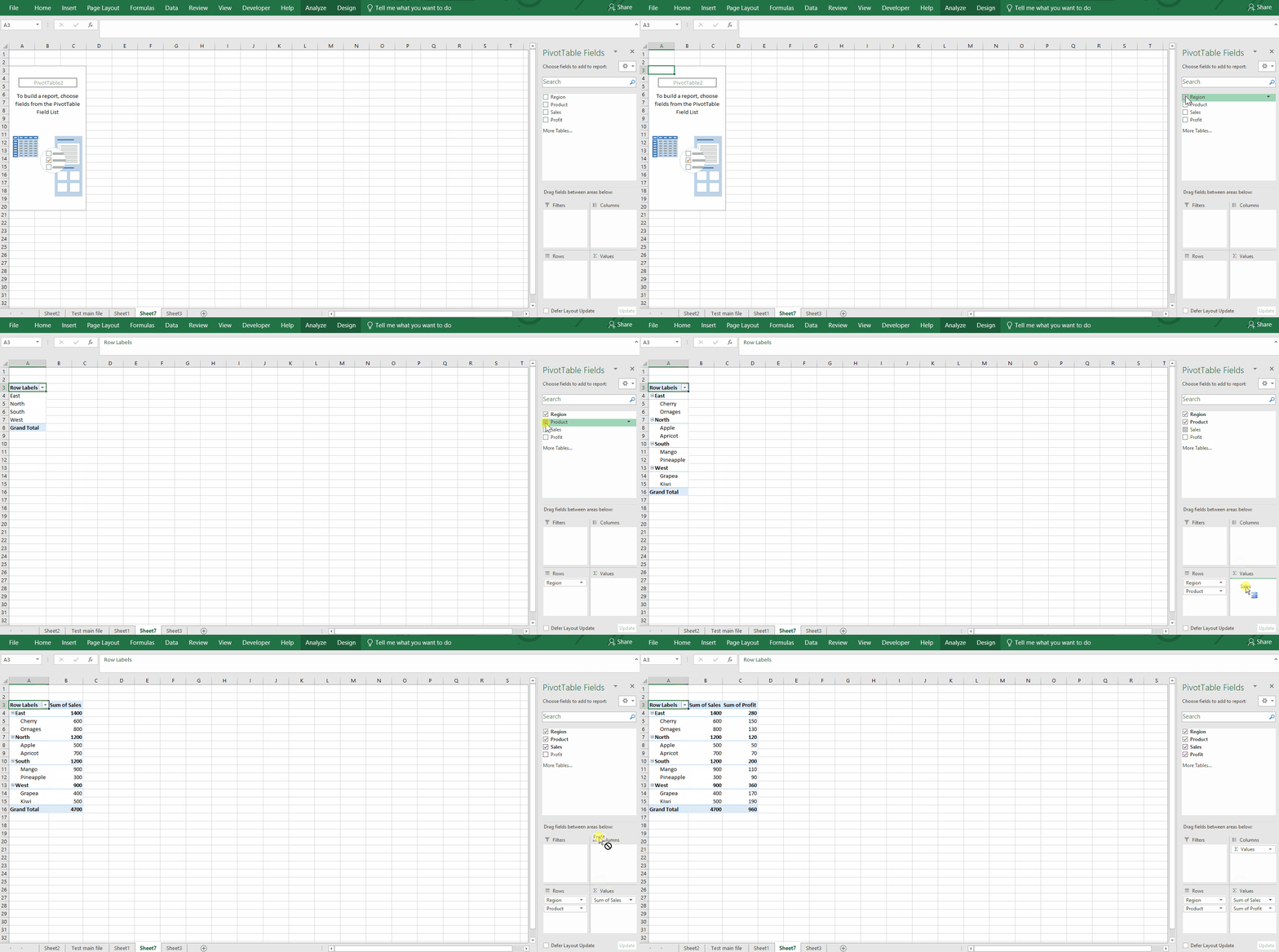
Step 2 – Select the headers for rows and values

– Select the region and product , drag into the ROWS section.
– Drag the Sales into the values section.
– Drag the Profit into the values section, As shown above;
Step 3 – Add the profit margin for each item

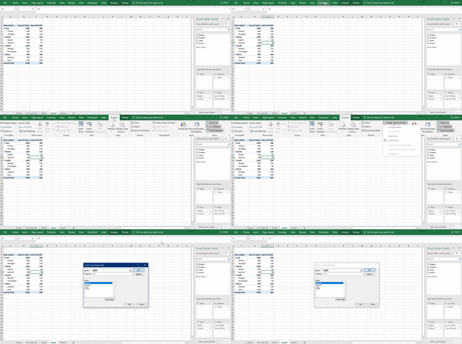
– Click on any cell in the Pivot Table.
– Go to (Pivot Table Tools) Analyze menu bar. Click on it .
– In the icon bar click on Fields, Items, & Sets . A drop down menu will appear.
– Click on the Calculated Field. A new dialogue box will appear, as shown below;
Step 4 – Go to the Insert Calculated Field dialog box

– Assign a name in the Name field.
– In the Formula field, insert the formula =Profit/Sales by clicking on the Insert Field button from the Fields box.
– Click ADD and then OK.
– Click on the newly added column name of percentage of profit a menu bar will appear.
– Click on the View fields settings.
– A dialogue box will open.
– Click on the Show Values As.
– Click on the drop down menu.
– Click on the % of the total column.
– Click OK .
– As soon as you press the enter key percentages will be visible , animation is right above;


