
How to calculate outliers in Excel
 By
SpreadCheaters
By
SpreadCheaters
You can watch a video tutorial here.
An important step in explanatory data analysis (EDA) is the identification of outliers. These are values in data that are extreme and far removed from the other data points. It is important to identify the outliers and, in most cases, remove them so that they do not adversely affect the results of the data analysis. If the dataset is small then it is easy to identify the outliers by sorting and looking at the data. If the dataset is large, then we can find the outliers using the InterQuartile Range (IQR).
Using the IQR, an outlier is defined as any value 1.5 times the IQR above the 3rd quartile (75th percentile) or 1.5 times the IQR below the 1st quartile (25th percentile). We will use the following functions in Excel to calculate the outliers:
1. QUARTILE(): this returns the value of a quartile of a range of numbers
a. Syntax: QUARTILE(range, quart)
i. range: the range of values to be evaluated
ii. quart: the quartile to be returned e.g. 1 for the first quartile
2. IF(): this evaluates a condition and returns a value depending on whether the condition is true or false
a. Syntax: IF(condition, true, false)
i. condition: the condition or statement to be evaluated
ii. true: the value to be returned if the condition is true
iii. false: the value to be returned if the condition is false
3. OR(): this determines if the conditions in a test are true or false
a. Syntax: OR(condition1, condition2….)
i. condition1: a logical test
Step 1 – Find the first quartile
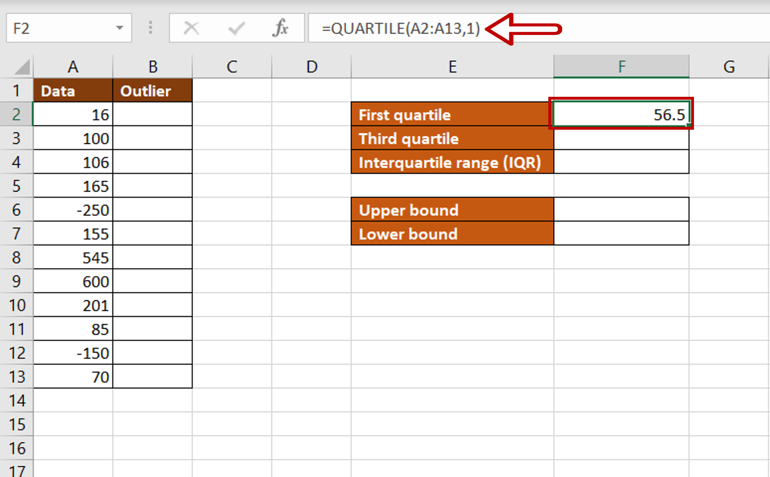
– Select the cell in which the value is to be displayed
– Type the formula using cell references:
= QUARTILE(Data, 1)
– Press Enter
Step 2 – Find the third quartile
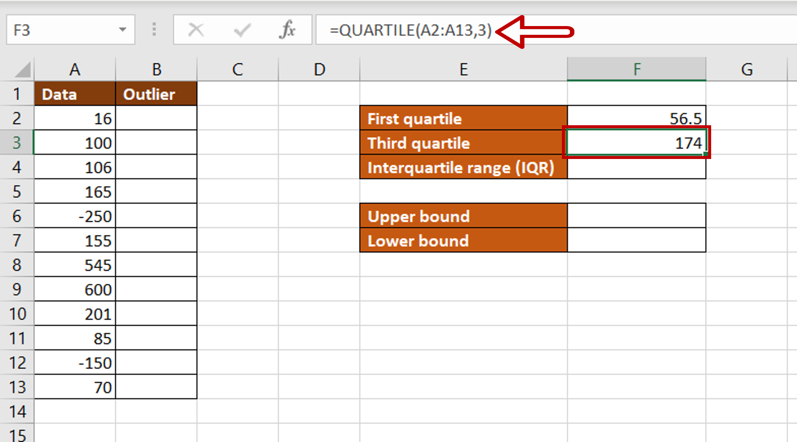
– Select the cell in which the value is to be displayed
– Type the formula using cell references:
= QUARTILE(Data, 3)
– Press Enter
Step 3 – Find the interquartile range (IQR)
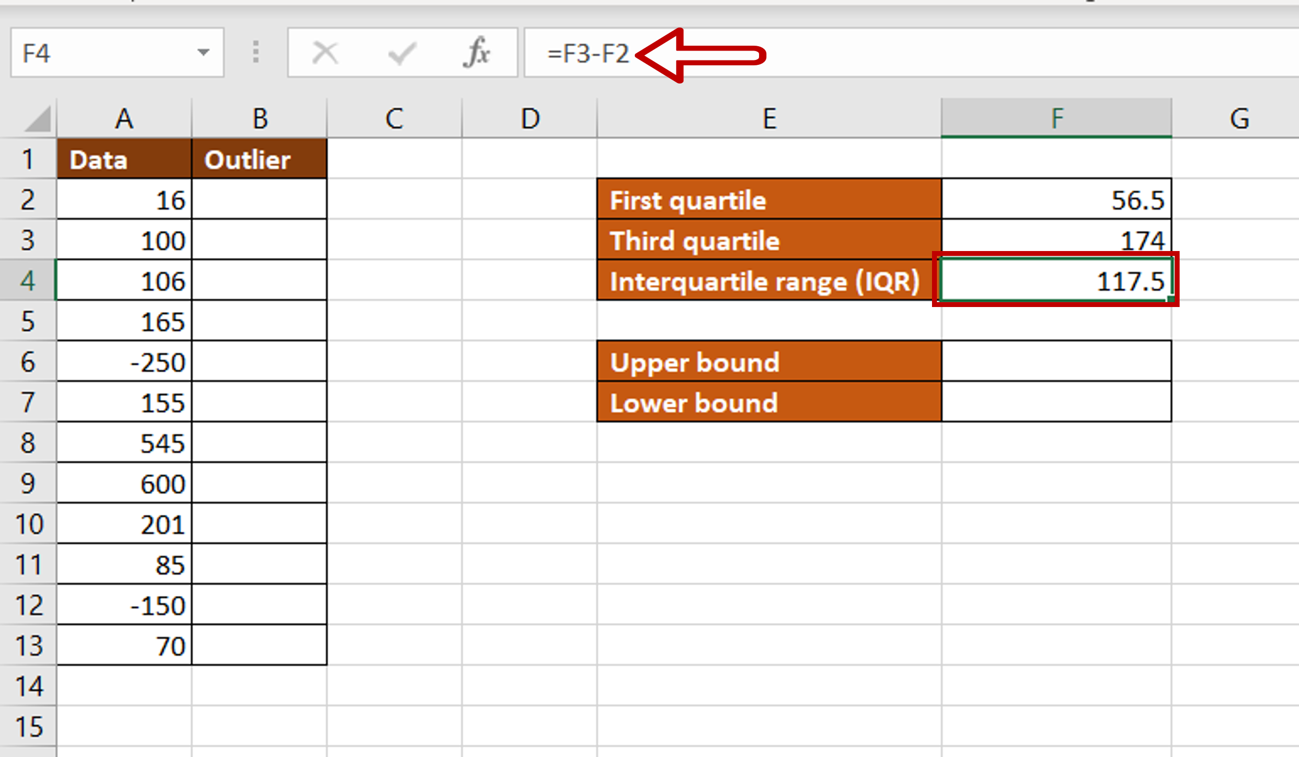
– Select the cell in which the value is to be displayed
– Type the formula using cell references:
= Third quartile – First quartile
– Press Enter
Step 4 – Find the upper bound
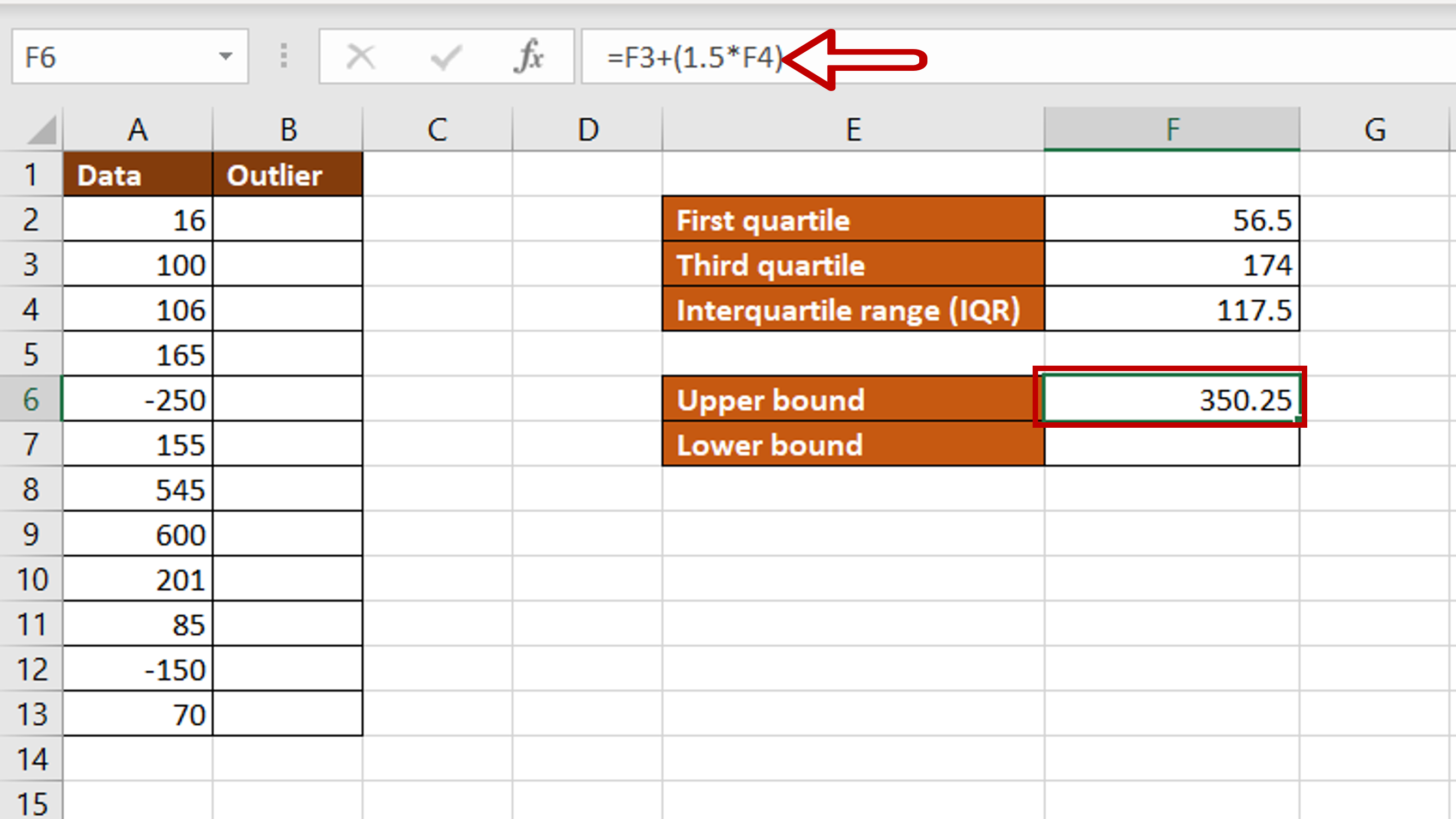
– Select the cell in which the value is to be displayed
– Type the formula using cell references:
= Third quartile + (1.5*IQR)
– Press Enter
Step 5 – Find the lower bound
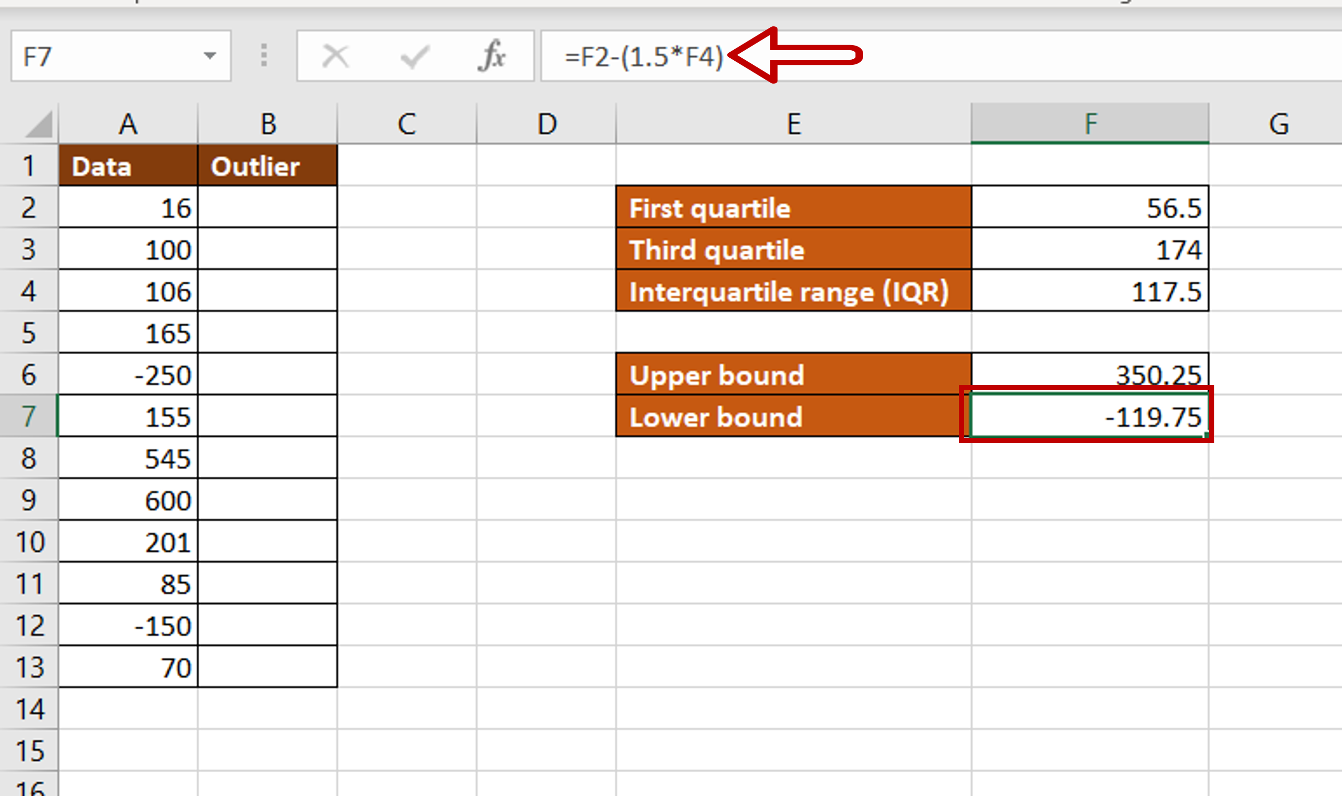
– Select the cell in which the value is to be displayed
– Type the formula using cell references:
= First quartile – (1.5*IQR)
– Press Enter
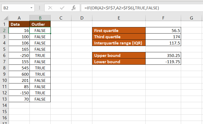
Step 6 – Create the formula for outlier detection
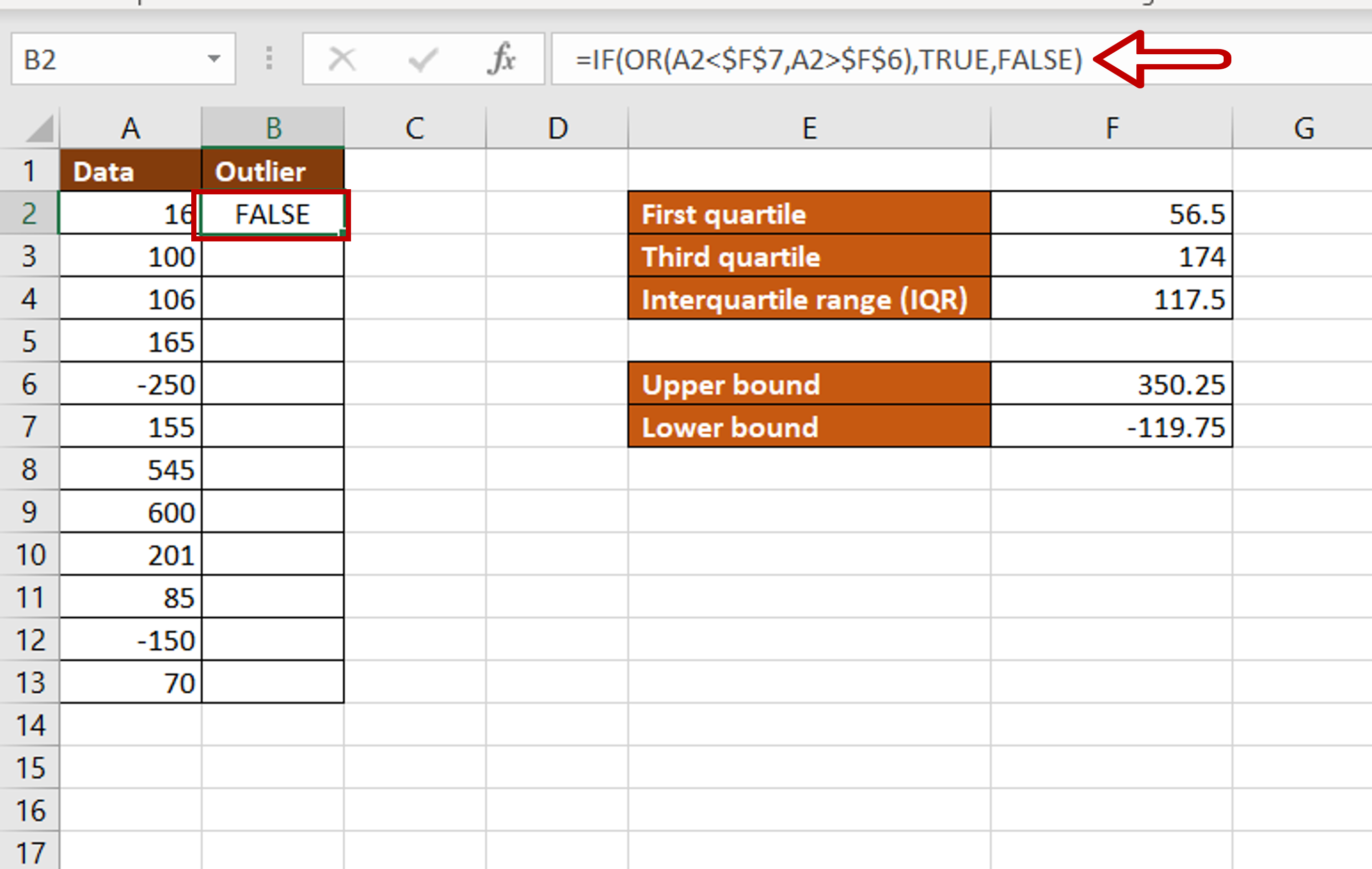
– Select the cell in which the value is to be displayed
– Type the formula using cell references:
= IF(OR(Data < $Lower bound$, Data > $Upper bound$),TRUE, FALSE)
– Add dollar signs ($) to the cell references of the Upper and Lower bounds to make them constant
– Press Enter
Step 7 – Copy the formula
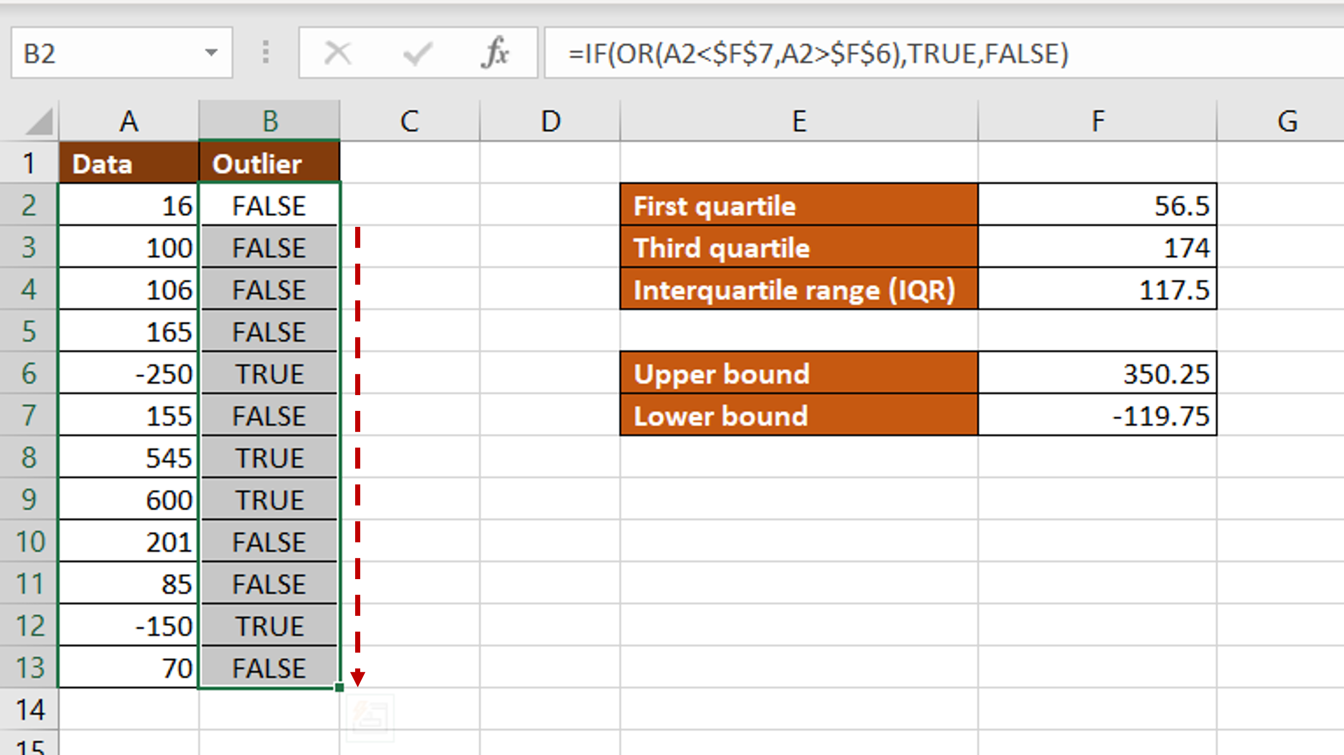
– Using the fill handle from the first cell, drag the formula to the remaining cells
OR
a. Select the cell with the formula and press Ctrl+C or choose Copy from the context menu (right-click)
b. Select the rest of the cells in the column and press Ctrl+V or choose Paste from the context menu (right-click)
Step 8 – Check the result

– The outliers have a value of ‘TRUE’ in the ‘Outlier’ column


