
How to calculate logarithmic regression in Excel
 By
SpreadCheaters
By
SpreadCheaters
Excel logarithmic regression is a statistical analysis technique used to model the relationship between two variables, where one variable is assumed to be dependent on the logarithm of the other variable. The overall importance of logarithmic regression lies in its ability to capture nonlinear relationships between variables.
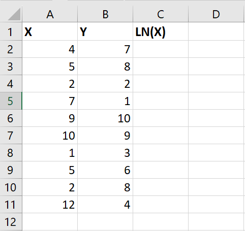
Step 1 – Click on the cell
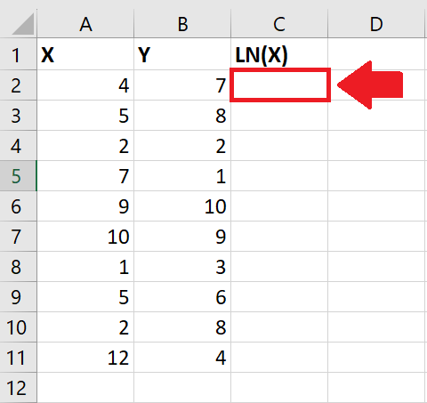
– Click on the first cell of the column, where you want to show the ln values
Step 2 – Type the Formula
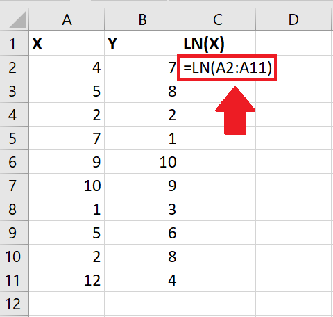
– After selecting the cell, type the following formula to get the log values:
– =LN(number)
– Where number is the value whose log is required (here it is A2:A11)
Step 3 – Press the Enter key
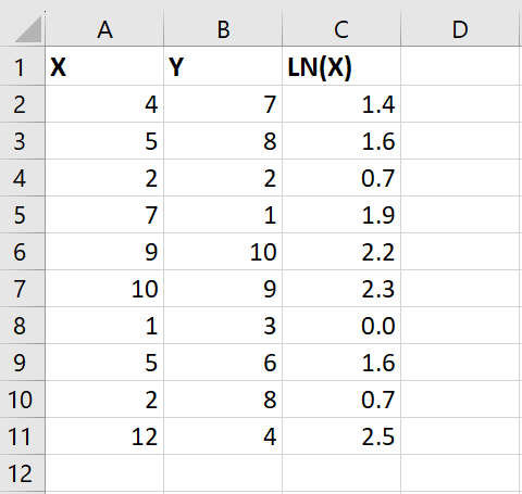
– After typing the formula, press the Enter key to get the log of numbers in the selected column
Step 4 – Click on the Data Analysis option
– After getting the log values, click on the Data Analysis option in the Analysis group of the Data tab and a dialog box will appear
Step 5 – Click on the Regression option
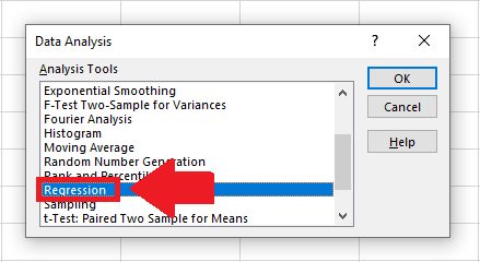
– In the dialog box, click on the Regression option
Step 6 – Click on OK
– Click on OK in the dialog box and a Regression dialog box will appear
Step 7 – Select the Y Range
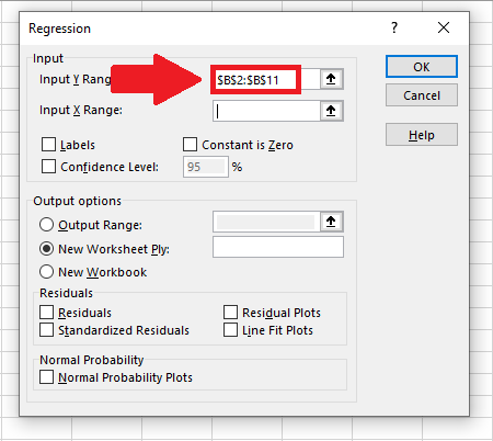
– Type the range of the Y-axis in the box next to the Input Y range option
Step 8 – Select the X Range
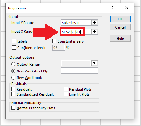
– Type the range of the X-axis in the box next to the Input X range option
Step 9 – Click on OK
– After typing the ranges, click on OK to get the result on the new sheet


