
How to calculate dot product in Microsoft Excel
 By
SpreadCheaters
By
SpreadCheaters
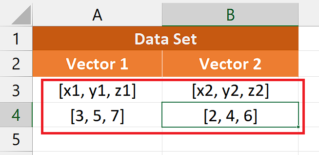
Let’s consider a scenario in which we have two three-dimensional vectors and we wish to calculate the dot product of these vectors. We have x1, y1, and z1 for the first vector’s components and x2, y2, and z2 for the second vector’s components.
Understanding the Function and its Syntax
In Excel, the SUMPRODUCT function is used to calculate the sum of the products of corresponding values in multiple arrays or ranges. It allows you to perform a weighted sum calculation by multiplying values from different arrays together and then summing those products. It is used here to calculate the dot product of vectors.
The syntax for SUMPRODUCT is as follows:
=SUMPRODUCT(array1, [array2], [array3], …)
array1 – The first array or range of cells to multiply.
array2, array3, … – Optional additional arrays or ranges to multiply.
The function multiplies the corresponding values from each array together and then adds up those products. The arrays must have the exact dimensions (same number of rows and columns) or they should be of equal length.
The dot product is a mathematical operation that calculates the sum of the products of corresponding elements in two vectors. The dot product can be used in various vector operations, such as determining the angle between two vectors or decomposing a vector into its parts. These operations can be valuable for tasks such as vector analysis, motion calculations, or signal processing.
Step 1 – Re-write the vector components
– Re-arrange the data as shown in the following animated image.
– This will help us to use these components of both vectors as inputs to the formula
Step 2 – Write the formula and implement it
– After selecting the cell, type = (equal sign) in the cell to initiate the formula.
– Then, type SUMPRODUCT and select the SUMPRODUCT Function by pressing the tab button.
– Now, select the first array or range of cells to multiply. For example, A6:A8
– After that, select the second array or range of cells to multiply. For instance, B6:B8.
– Now, add a closing parenthesis.
– After following the above steps, your formula would look like this
=SUMPRODUCT(A6:A8,B6:B8)
– Then, press Enter and the dot product will be calculated.


