How to Calculate Compound Interest for Compounding Period on a daily basis for one year in Excel
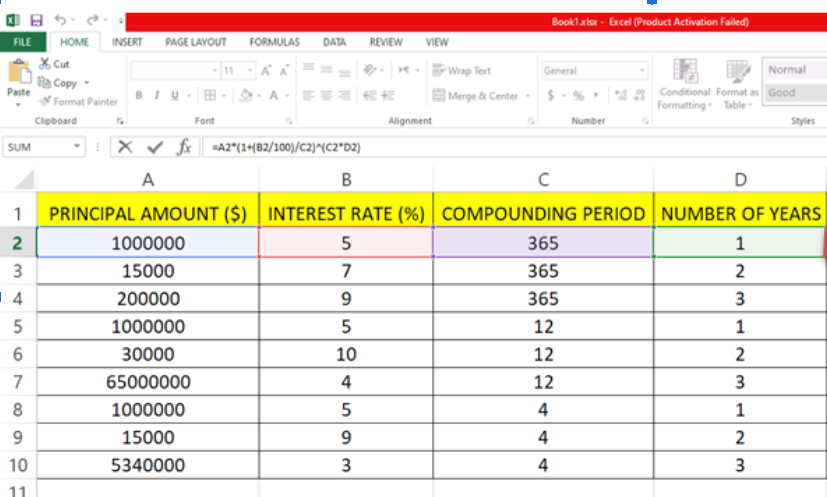
In this tutorial we will learn how to calculate Compound Interest using Excel. Here we have a dataset in which Principal Amount ($), Interest Rate (%), Number of Years Compounding Period is given. In this dataset there are three different types of values for Compounding Period (365 for days in year, 12 for months in year and 4 for quarters in year).There are nine values for each column in this dataset. For finding Compound Interest ($) we first have to find Total Interest ($), formula and steps to implement the formula are given above.
Follow the steps given below to find Interest and Compound Interest.

Microsoft Excel is a spreadsheet program that is used to manage and analyze data. Excel is widely used in various fields and industries for tasks such as financial analysis, budgeting, project management, and more. It offers a flexible and versatile platform for data analysis, reporting, and decision-making.
Step 1 – Type the formula to calculate Interest
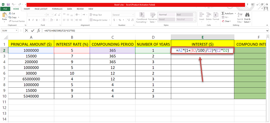
– For finding the interest we have to use this general formula :
I= A(1+(r/100)/n)nt
I= Interest($).
A = Principal Amount($).
r = Interest rate(%).
n = Compounding Period (Set it to 365 days for interest based on daily basis).
t = Number of years.
– According to the given dataset this formula for Excel can be written as =A2*(1+(B2/100)/C2)^(C2*D2).
– We’ll write this formula in Cell E2 in our case.
Step 2 – Find Interest for all other values
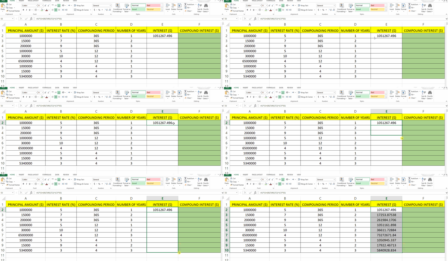
– Move the cursor to the cell in which you typed the formula and then drag it down to the other cells and Excel will automatically calculate the other values using the same formula.
– In this example cell E2 is selected and it is dragged till E10.
Step 3 –Type the formula for finding Compound Interest.
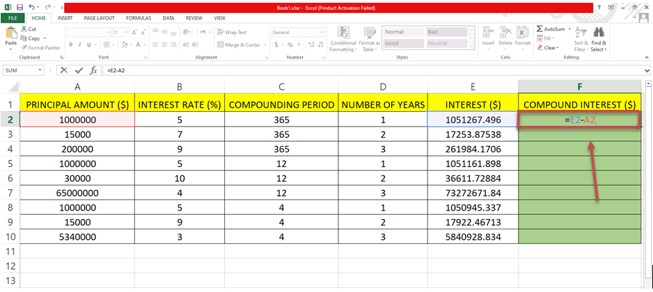
– We have already calculated interest and now will find Compound Interest.
– To find Compound interest we have to subtract the Principal Amount from the Interest.
– Formula:
C= I-A
C = Compound Interest($).
I = Interest($).
A = Principal Amount($).
– In this Dataset Column A is for Principal Amount and column E is for Interest.
– The formula for Excel will be =E2-A2.
– The cell location that you typed in the formula will get highlighted which will help you check which cell is being selected (E2 and A2 is highlighted in the image above).
Step 4 – Find Compound Interest for all other values
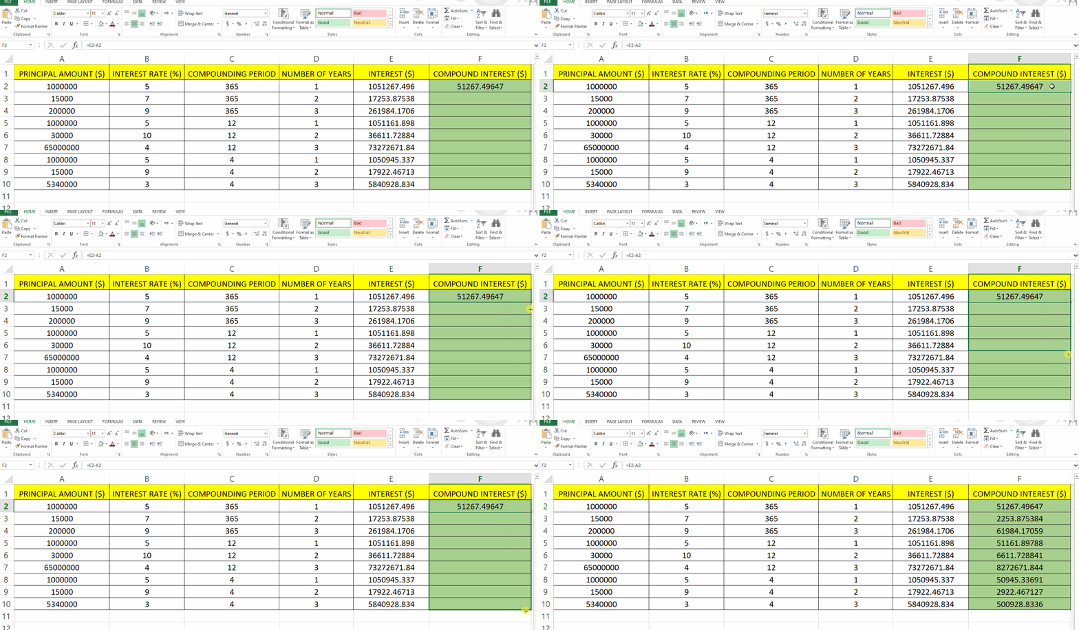
– Move the cursor to the cell in which you typed the formula and then drag it down to the other cells and Excel will automatically calculate the other values using the same formula.
– In this example cell F2 is selected and it is dragged till F10.


