
How to calculate annualized returns from monthly returns in Excel
 By
SpreadCheaters
By
SpreadCheaters
Page last updated:
04/01/2023 |
Next review date:
04/01/2025
You can watch a video tutorial here.
Calculating the annualized return of an investment is a way of understanding how well the investment is doing. This can be done using the monthly returns of the investment. Excel does not have a function for this calculation but you can create the formula in Excel.
The formula for calculating the annualized return is:
- Annualized return = (1+R)^12-1
- R is the monthly rate of return
This can be applied if the rate of return is the same for each month. If it is not, then (1+R) is multiplied for each month.
Option 1 – The rate is the same for each month
Step 1 – Create the formula
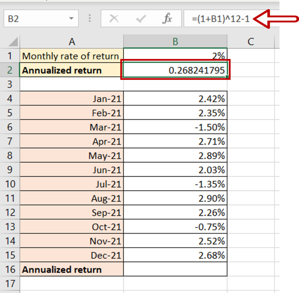
- Select the cell in which the result is to appear
- Type the formula using cell references:
- =(1+Monthly rate of return)^12-1
- Press Enter
Step 2 – Format as a percentage
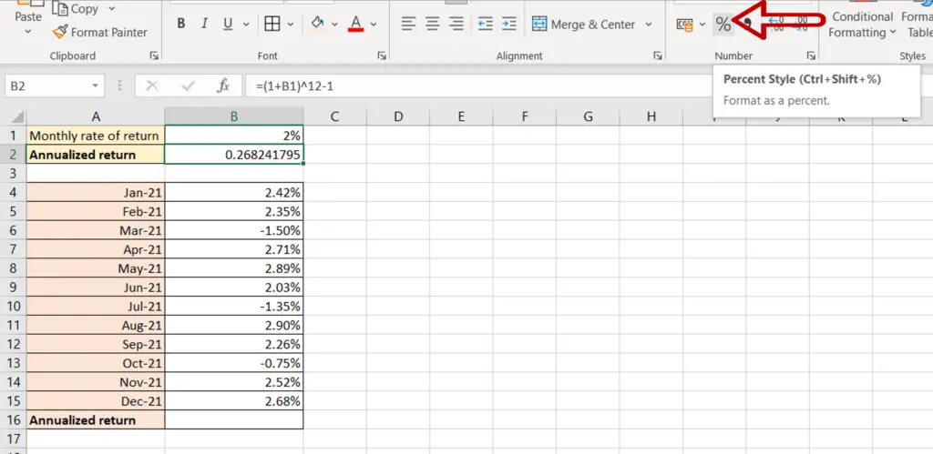
- Click the Percent Style button on the ribbon
Step 3 – Check the result
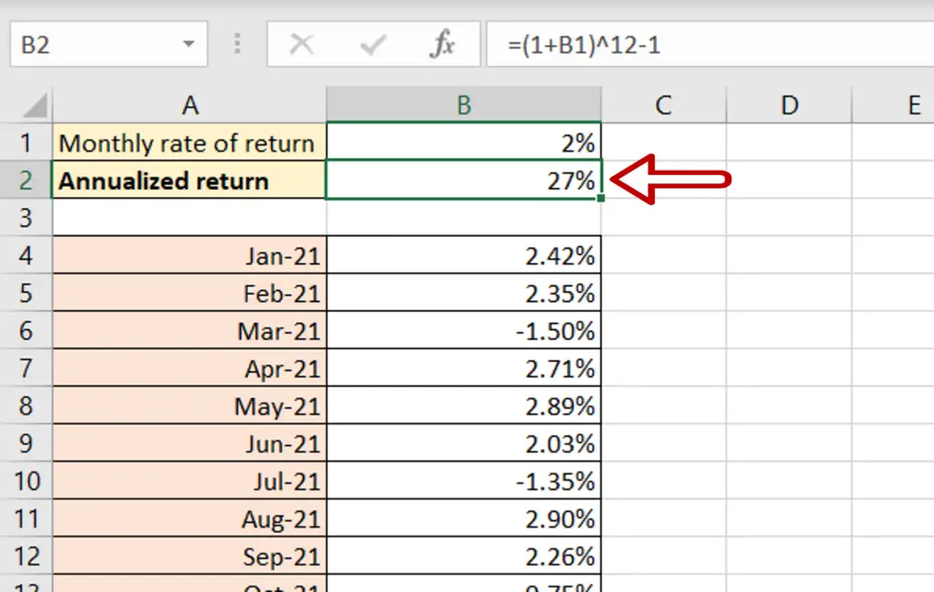
- The annualized return is displayed
Option 2 – The rate is different for each month
Step 1 – Create a temporary column
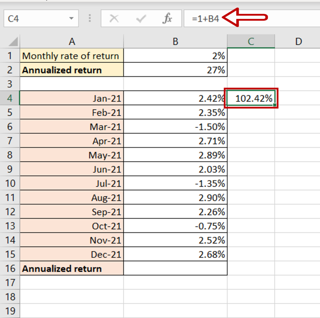
- Select the cell next to the return for Jan 2021
- Type the formula using cell references:
=1+Monthly rate of return
- Press Enter
Step 2 – Copy the formula
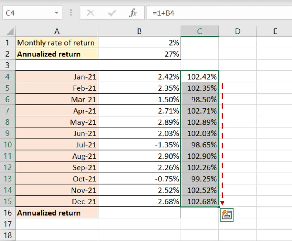
- Using the fill handle from the first cell, drag the formula to the remaining cells
OR
- Select the cell with the formula and press Ctrl+C or choose Copy from the context menu (right-click)
- Select the rest of the cells in the column and press Ctrl+V or choose Paste from the context menu (right-click)
Step 3 – Create the formula
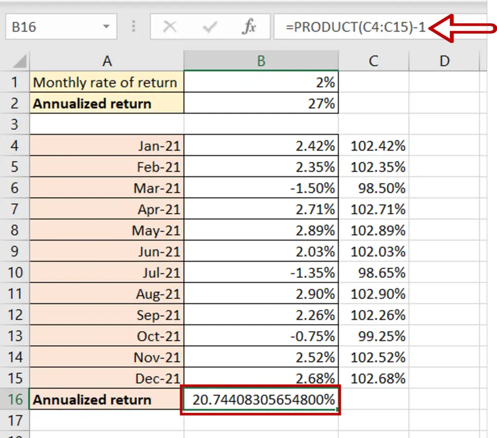
- Select the cell where the result is to appear
- Type the formula using cell references:
- = PRODUCT(temporary column)-1
- Press Enter
Step 4 – Check the result
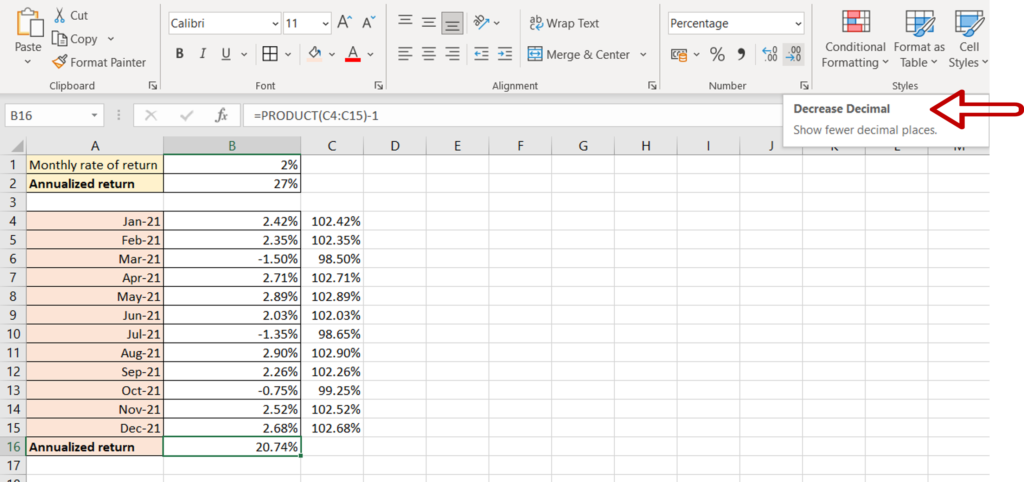
- Press the Decrease Decimal button to reduce the number of decimal places
- The annualized return is displayed


