How to calculate age in Excel in DD/MM/YYYY

Demography is the science of populations. Researchers use demographic information to describe the sample of the target population. One of the most important demographic information a researcher needs is age. If you’re a researcher, then you’ll need to know how to calculate age in Excel using birthdays.

There are many ways you can calculate the age. The three most accurate in achieving this are the following formulas written below:

• =YEAR(NOW())-YEAR(B3)

• =INT(YEARFRAC(B3,TODAY()))
• =DATEDIF(B3,NOW,”Y”)

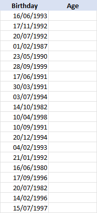
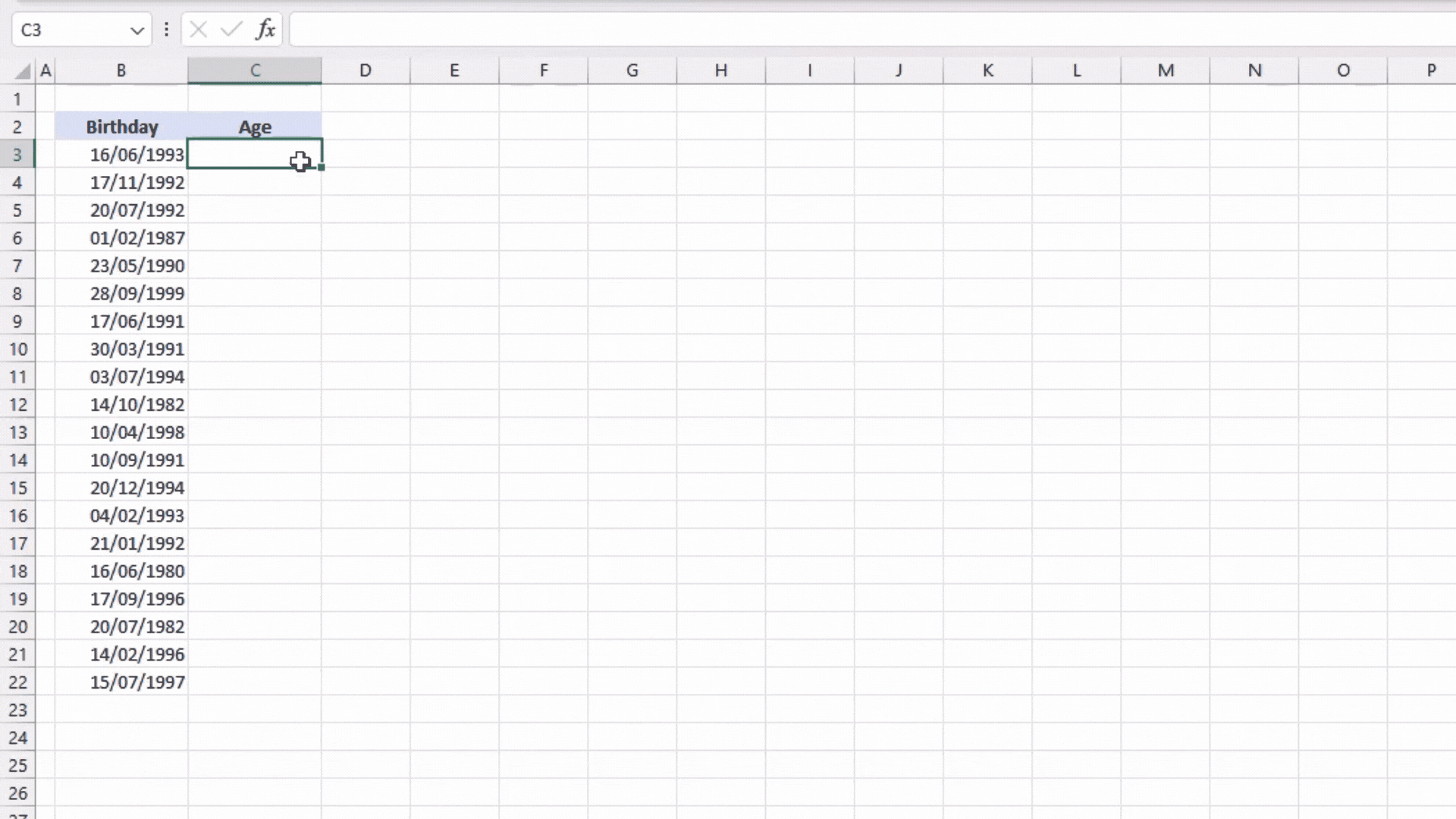
We will learn each formula with a step by step guide provided in this tutorial. We will use the table above as our example.

=YEAR(NOW())-YEAR(B3)

This formula means we are subtracting the year of the birthday to the year now. Our formula contains two functions: the YEAR function, and the NOW function. YEAR function is used to calculate the year corresponding to a date. While the NOW function returns the current date and time. 

Now let’s see how the combination of this function can give us the age with just a birthday.

Step 1 – Construct our minuend

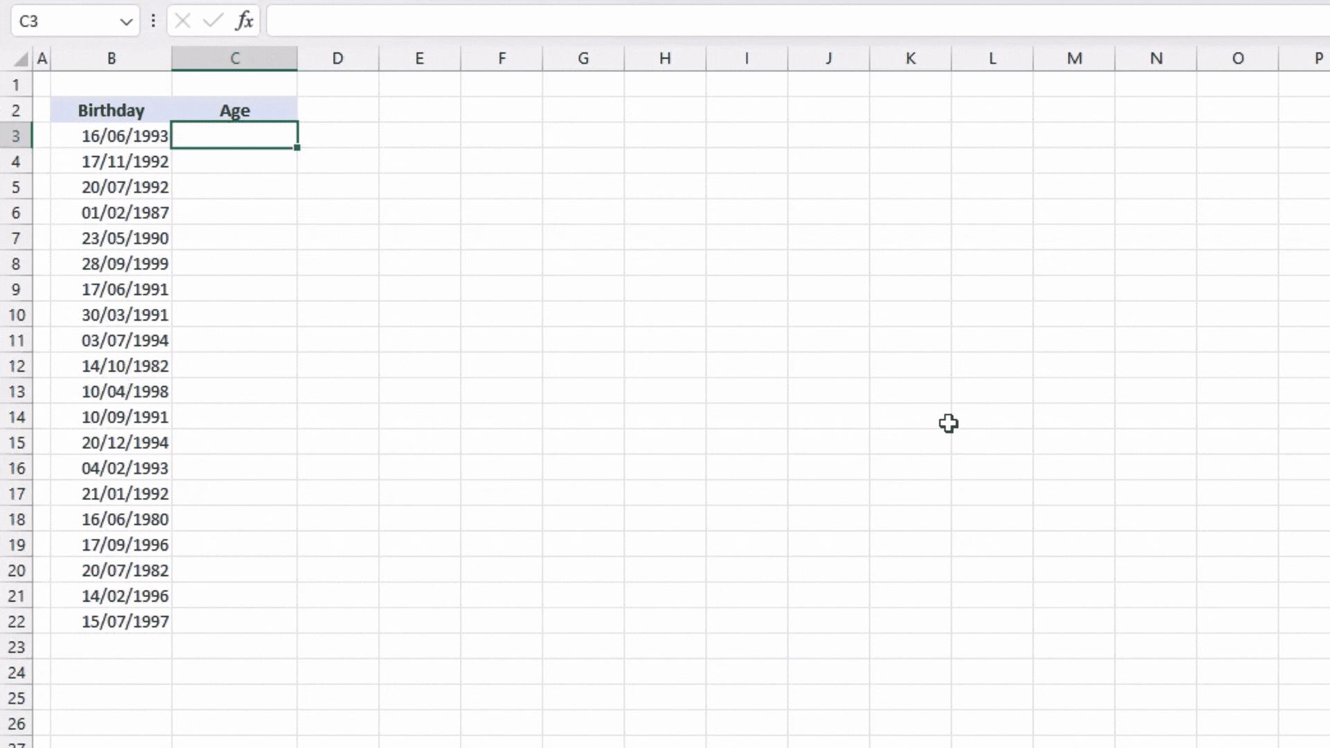
• Enter the YEAR function.
• Our minuend will be the current year so we will be using the NOW function as our argument.
• Close the NOW and YEAR function simultaneously by adding two close parenthesis “)” at the end of our minuend.

=YEAR(NOW))

Step 2 – Construct our Subtrahend

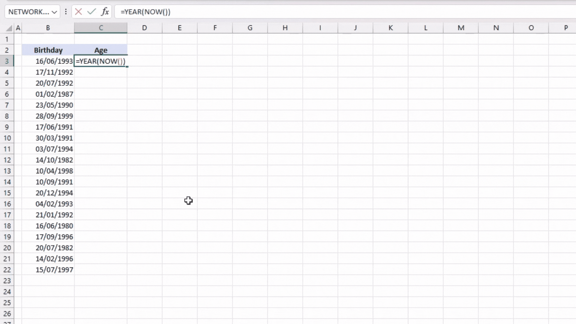
• Put a minus sign “–” right after the last close parenthesis “)”
• Enter another YEAR function.
• The birthday should be our subtrahend thus we will select the cell that contains the birthday within the row as our argument. 
• Close the YEAR function by adding a close parenthesis “)” at the end.
• Hit ENTER on your keyboard.

=YEAR(NOW))-YEAR(B3)

Step 3 – Extend the formula

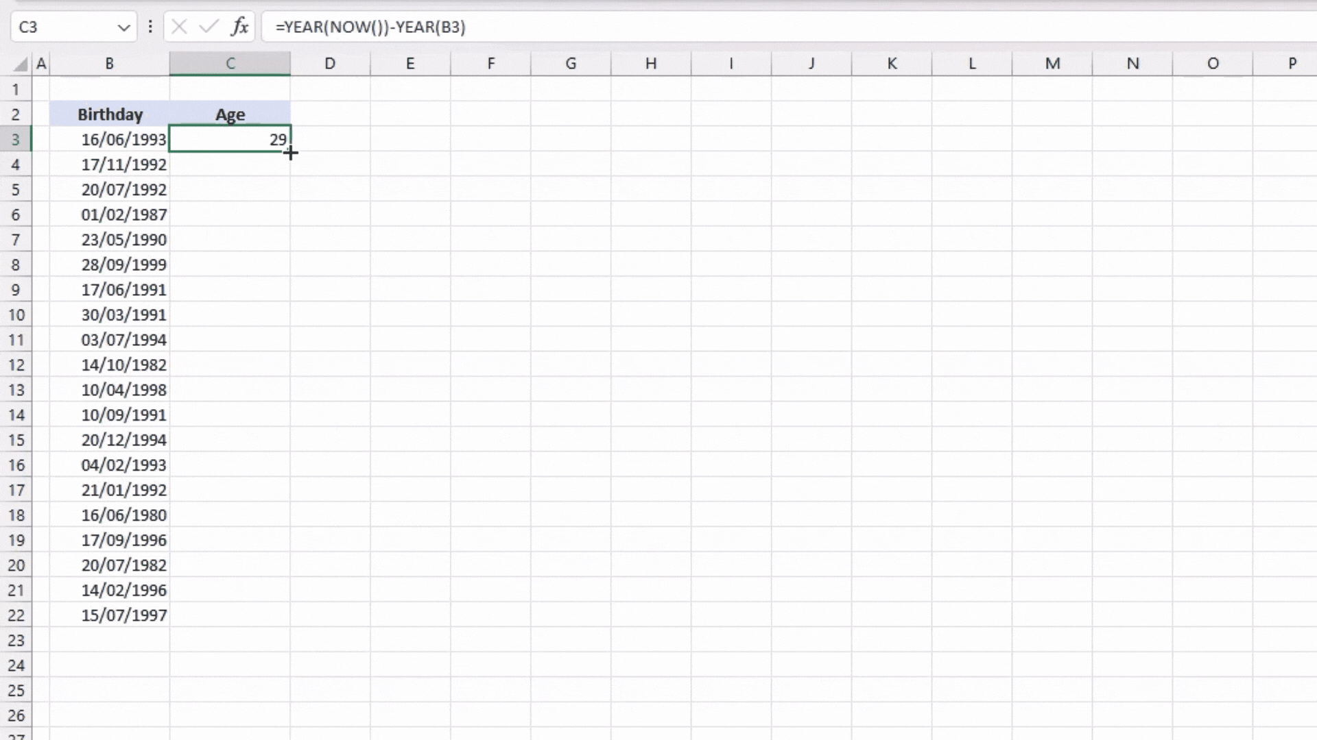
• Extend the formula by dragging the small green square located in the lower right of the cell we were working on.

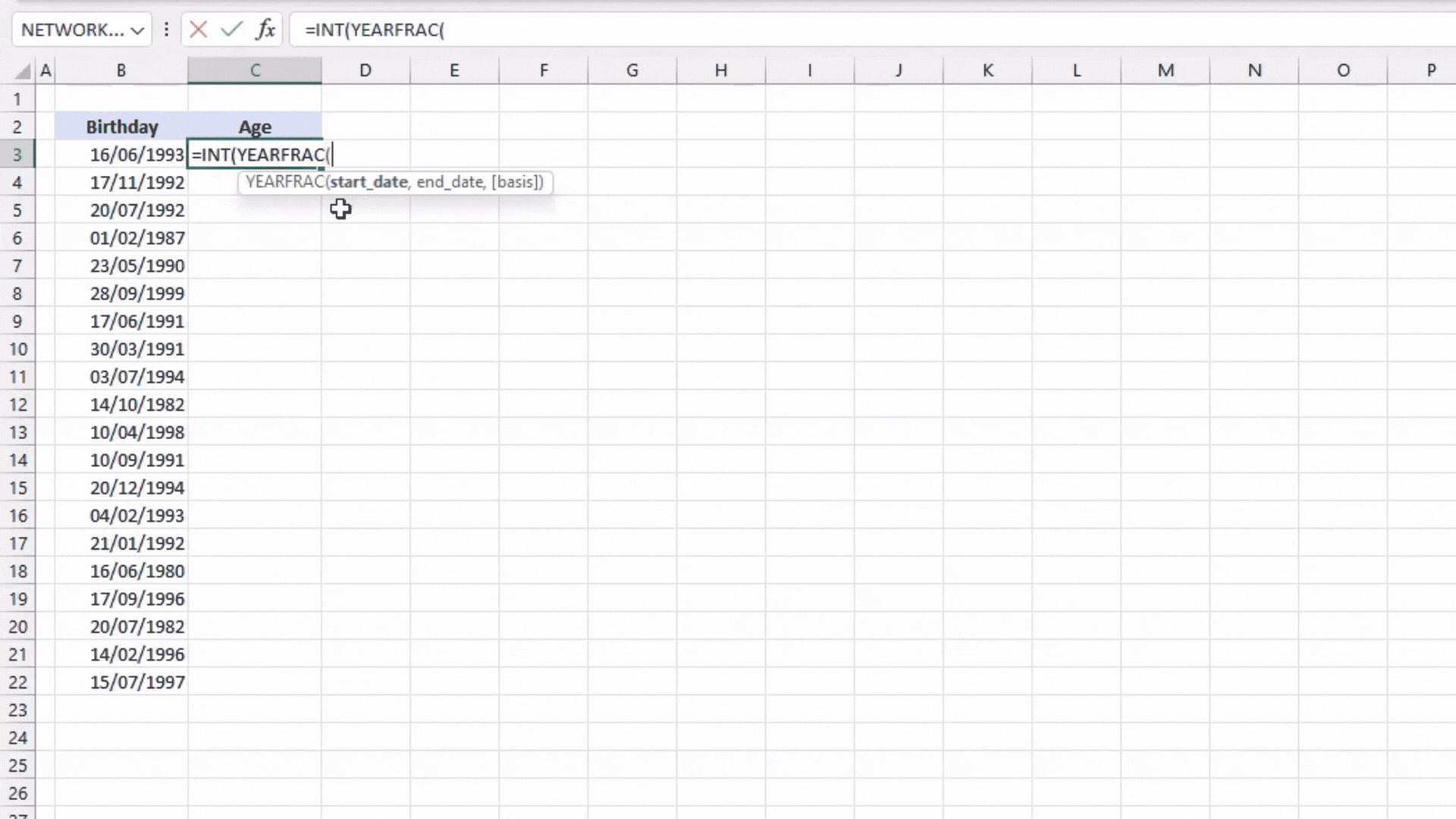
=INT(YEARFRAC(B3,TODAY()))

We will be using a different set of functions for this formula: INT function, YEARFRAC function, and TODAY function. INT function is used to round a number down to the nearest integer. The YEARFRAC function is used to calculate the number of days between two dates in year fraction. It contains three arguments: start_date, end_date, [basis]. The arguments start_date and end_date should be a value recognized by Excel as date. It could only be entered in Excel using the DATE function or as a reference to a cell that contains a date. While the argument [basis] is an optional argument. It has a preemptive selection of basis on how you want to count the days. And the last function we will use is TODAY function. Unlike the NOW function, it only returns the current date without the current time.

The meaning of this formula is that we are getting the difference between today’s date and the given birthdate. But since the function YEARFRAC is returning a number in decimal form, we need to use the INT function to round it down to the nearest integer.

Now, let us combine the three functions we just learned to create a formula in determining the age using birthdays.

Step 1 – Enter the functions

• The first function to be entered into the cell is the INT function.
• Upon opening the INT function, we will enter the YEARFRAC function.

=INT(YEARFRAC(

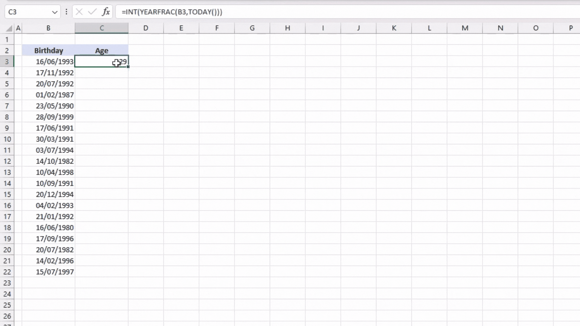
Step 2 – Determine the arguments

• We will use the birthdays on Column B as our start_date. 

• Then we will use the current date as our end_date, so TODAY function will be our second argument.
• We are now complete with TODAY, YEARFRAC and INT functions. There should be three close parentheses “)” at the end of our formula.
• Press ENTER on your keyboard.

=INT(YEARFRAC(B3,TODAY()))

Step 3 – Extend the formula

• Drag the formula down to apply the same formula to every row and get the age of each birthday.

=DATEDIF(B3,TODAY(),”Y”)

The DATEDIF function is not a standard function on Excel thus it cannot be found in the functions library. It will not show up in the recommendations when you type in “DATEDIF” and it will not also open its arguments once you press TAB on your keyboard. Microsoft doesn’t promote the use of this function as it gives incorrect results in a few circumstances. However, it is not the same with calculating age. It can give us an accurate result so we can use this function. But because of its invisibility from the functions library, we need to thoroughly understand the syntax of this function.

The DATEDIF function has three arguments: start_date, end_date, and unit. The meaning of this function is getting the difference of two dates (start_date and end_date) according to the chosen time unit (unit). There are different selections for the unit. Each of them are in the table below:

Unit	Returns
“Y”	Complete number of year between the two dates
“M”	Complete number of months between the two dates
“D”	Complete number of days between the two dates
“MD”	*Number of days between two dates, ignoring year and months
“YM”	Number of months between two dates, ignoring years and days
“YD”	Number of years between two date, ignoring months and days

    *This unit gives an incorrect result.

Our formula means we are getting the difference between two dates in terms of years. Now that we know the arguments, we can now create the formula.

Step 1 – Writing the formula

• We have to write the function manually. Type “=DATEDIF(“ on the cell or formula bar.
• The start_date will be the birthday so we will select B3
• We will choose the current date as our end_date thus we enter TODAY function.
• We want the complete number of years thus “Y” will be our third argument.
• Close the formula and hit ENTER.

=DATEDIF(B3,TODAY(),”Y”)

Step 2 – Extend the formula.

• Just like in every other process, extend the formula down to the bottom of our list.

There you have it! You just learned the two most accurate and easiest formulas on getting the age using the birthday in DD/MM/YYYY format. It saves you time especially when you have thousands of items in your list. Hope we helped you with your research.