How to calculate 90 days of employment in Excel

Most of the companies use Employee Referral Program for finding talents. It is a program for the existing employees to recommend candidates within their existing networks. It is compensated through a Referral Bonus. But it’s not always when your recommended colleague gets hired you’ll be entitled to it. Recruitment teams often set rules on when the referrer will be eligible to get their Referral Bonus. Most of the time, it depends on the number of days of employment of the referee. If you’re a part of the recruitment team, then you’re on the right page. We will learn how to calculate 90 days of employment and a way to track it.

Let us first learn the functions that we’re supposed to use to achieve this.

TODAY Function

=TODAY()

TODAY function is under ‘Date and Time’ functions of Excel. Its function is to get the current date. It doesn’t require any argument. However, just like any other function, a parenthesis will open after you enter the function. You just have to close it without any arguments inside the parentheses. Additionally, the return of this function updates continuously to the current date every time you open the worksheet.

WORKDAY Function

=WORKDAY(start_date,days,[holidays])

WORKDAY function is also categorized under Excel’s ‘Date and Time’ functions. It returns with a date before or after the number of working days you set. The syntax of the function is written above. The first argument, start_date, is a date value. It can be referenced to a cell that contains the date value or be entered using the DATE function. The next argument, which is days, is the number of workdays you set to be added to the start_date. It can be a positive or negative value which returns a date in the future or in the past, respectively. And [holiday], the last argument, is optional. It specifies an array of dates that are to be considered as non-workday.

Now let’s go into the steps.

Step 1 – Set the current date and  the number of days

• It is important to put these details in a secured area within the worksheet to avoid being accidentally deleted. In our case, we will put these above our list.
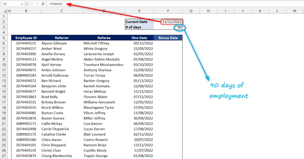
• Use the TODAY function to get the current date on cell F2
• Put the number of days, 90, on cell F3

Step 2 – Input the formula

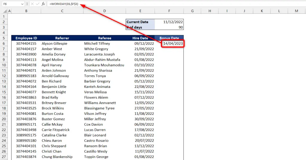
• Go to the first item in our list which is cell F6
• Input the function WORKDAY
• We will use the ‘Hire Date’ on Column E as our start_date
• The days argument we will input is 90 on cell F3. Take note that we should make an absolute reference to cell F3. You can manually put dollar signs on each side of the character ‘F’, or simply press F4 on your keyboard.
• Leave [holiday] blank then hit ENTER.

=WORKDAY(E6,$F$3)

Step 3 – Extend the formula

• Extend the formula by giving the fill handle a double-click.

Now that we have the dates, let us organize our list and apply some conditional formatting so it will be easy for us to track who is on their 90 day of employment.

Step 1 – Sort the date

• It is much easier to look at this long list of dates if it is arranged from oldest to newest.
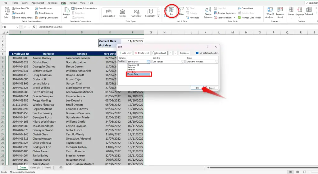
• Click on any part of our list, go to Data tab and select the Sort under the ‘Sort & Filter’ group.
• Sort the ‘Bonus Date’ on Column F from oldest to newest.

Step 2 – Conditional Formatting

• From cell E6, hold the keys CTRL and SHIFT, then press Down Arrow twice. In this way, we are going to apply the conditional formatting on the future referrals that will be listed in here.
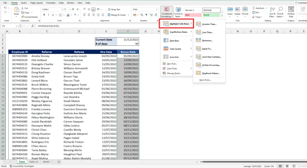
• Go to Home tab and click on Conditional Formatting on the ‘Styles’ Group.
• Hover your pointer on ‘Highlight Cells Rules’

Step 3 – Indicator for due today

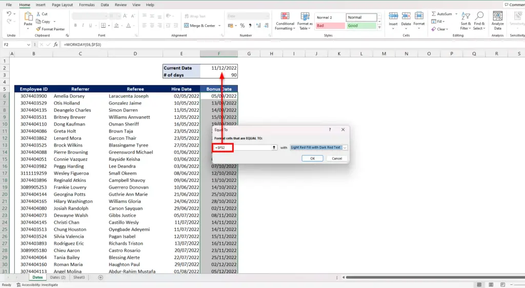
• From the hovered state of ‘Highlight Cells Rules’, click on ‘Equal To…’
• We want an indicator on the dates that is due on the current date so select the cell where we input the TODAY function, cell F12
• Format it on how you want to display these dates. In our excel, we will chose from the format available

Step 4 – Indicator for dates that already past

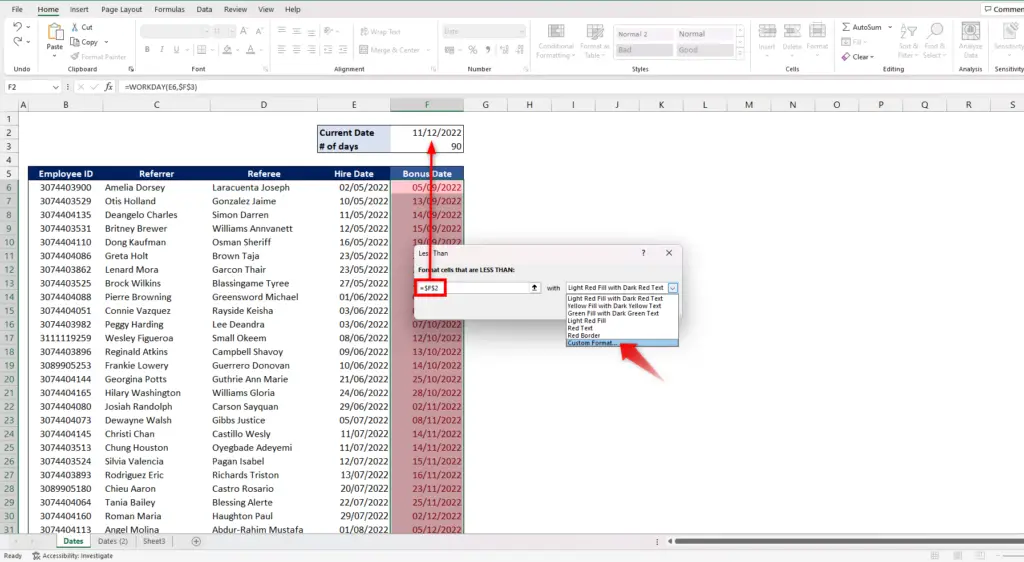
• Hover again on ‘Highlight Cells Rules’, click on ‘Less Than…’
• Select cell F2
• And format it how you want it to display. In the example, we want it to look greyed out so we chose to custom format

Step 5 – Indicator for dates that are due in three days

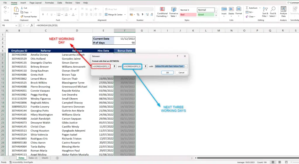
• For the last time hover on ‘Highlight Cells Rules’, and this time click on ‘Between…’
• We want it to change color if the date falls between the next working day and the next three working days. Thus, we should input these formulas in the boxes. It can be interchangeable.

=WORKDAY($F$2,1)

=WORKDAY($F$2,3)

• And format it how you want it to display. But in the example, we used the format available

Finally, we have the list of dates with indicators. In our example, this is what our list should look like on December 16, 2022. 

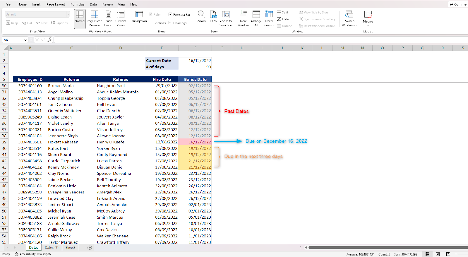
With the formatting, it is now simpler to keep track of the dates and prevent missing any on your lengthy list.