How to build a two-level custom sort in Microsoft Excel

A two-level custom sort means that you want to sort your data by two criteria, such as sorting first by the values in one column, and then by the values in a second column.

In this tutorial, we will learn how to build a two-level custom sort in Microsoft Excel. Sorting is one of the most basic tasks in Microsoft Excel that can be achieved by both the Sorting options in the Home tab as well as the Sorting tab in the Home tab.

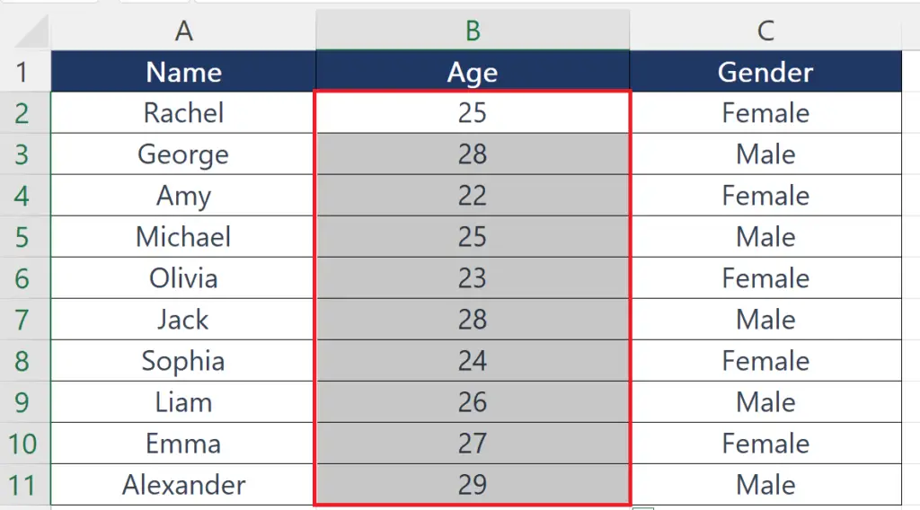
Let’s say, we have a data set that displays the names, ages, and gender of some employees of a firm. We want to sort the data first by age in ascending order and then by names in descending order.

Method 1: Utilizing the Sort Option in the Data 

Step 1 – Select the Data

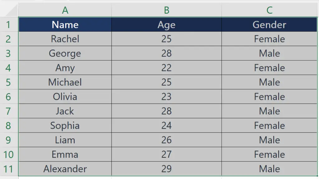
• Select the data on which you want to apply a two-level custom sort.

Step 2 – Locate the Data Tab

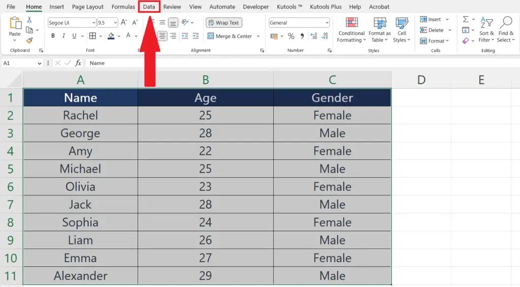
• Locate the Data tab in the menu bar.

Step 3 – Perform a Click on the Sort Button

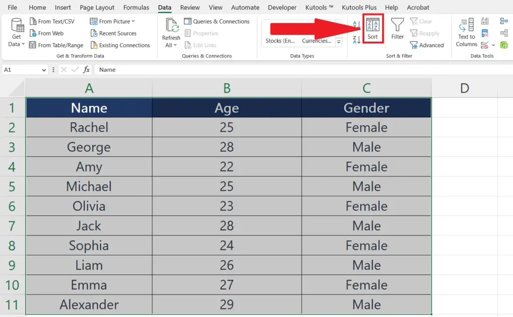
• Perform a click on the Sort button in the “Sort & Filter” section.

Step 4 – Choose the Sorting Options for the First Sort

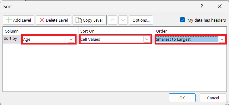
• Choose the sorting options for the first sort in the dialog box.
• In this case, we will choose the “Age” column from the “Column” drop-down menu and choose the “Smallest to Largest” option in the “Order” drop-down menu.

Step 5 – Perform a Click on the “Add Level” Button

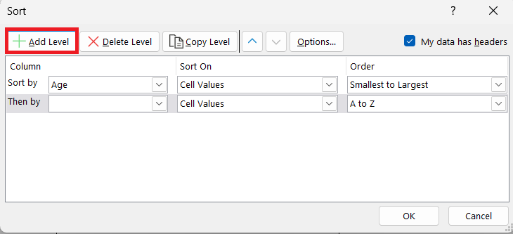
• Perform a click on the “Add Level” button.

Step 6 – Choose the Sorting Options for the Second Sort

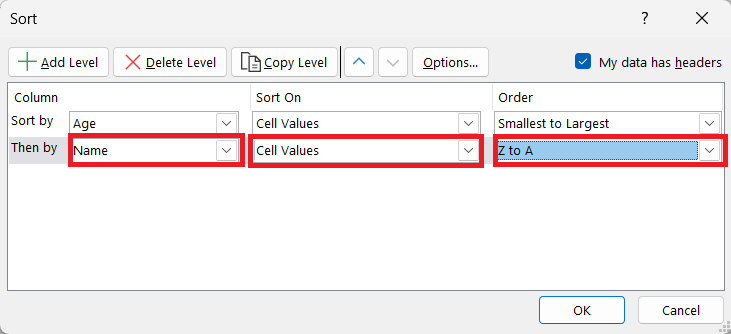
• Choose the sorting options for the second sort in the dialog box.
• In this case, we will choose the “Name” column from the “Column” drop-down menu and choose the “Largest to Smallest” option in the “Order” drop-down menu.

Step 7 – Hit the OK Button

• Hit the OK button in the dialog box.

Method 2: Utilize the Sorting Options in the Home Tab

Step 1 –   Select the First Column to Sort the Data

• Select the first column to sort the data.

Step 2 – Locate the “Sort & Filter” Button

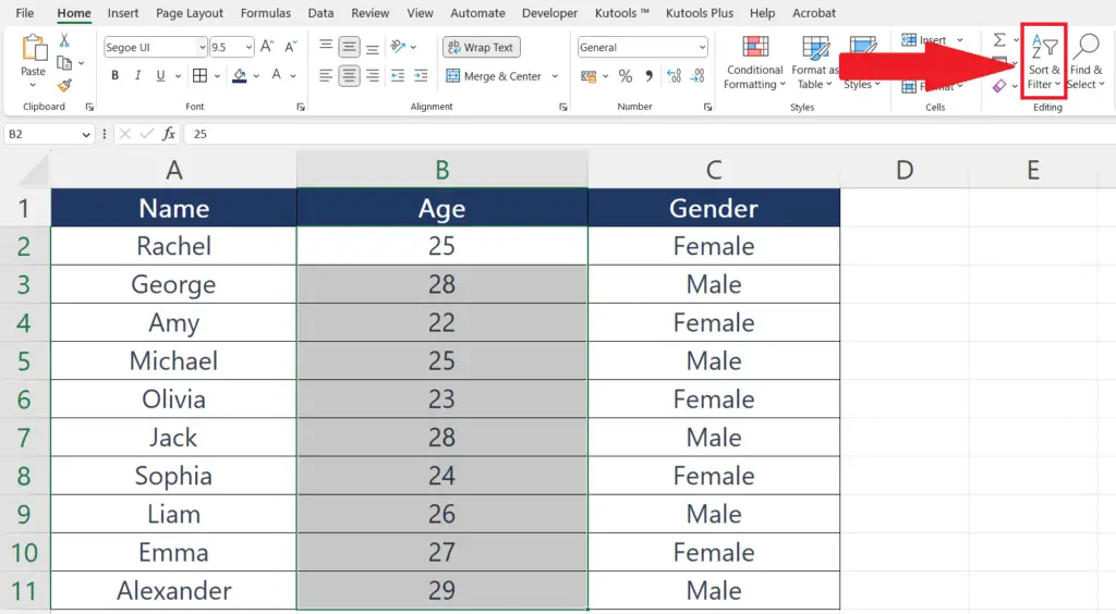
• Locate the “Sort & Filter” button in the Home tab.

Step 3 – Perform a Click on the “Sort smallest to largest” Option

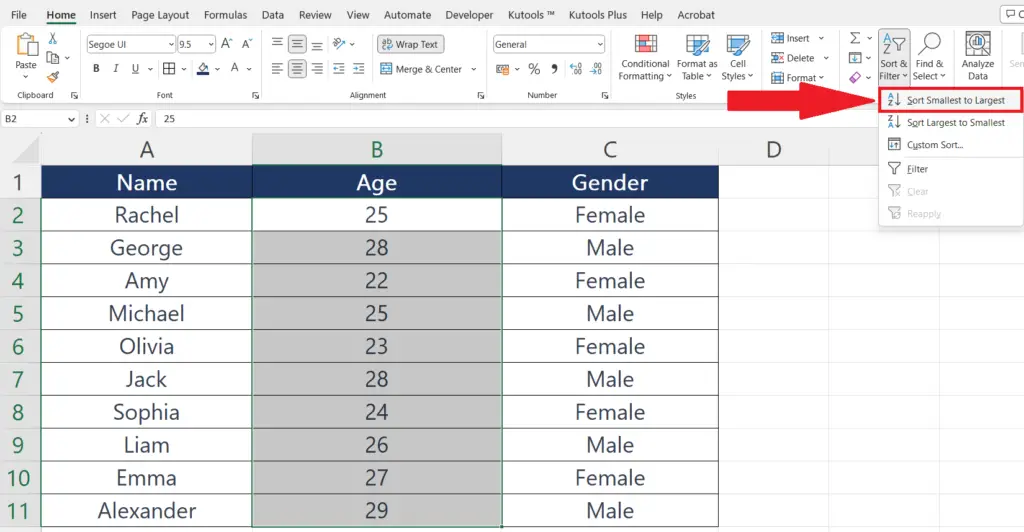
• Perform a click on the “Sort smallest to largest” in the drop-down menu.
• Choose the “Expand the Selection” option in the dialog that appears and click on OK.

Step 4 –   Select the Second Column to Sort the Data

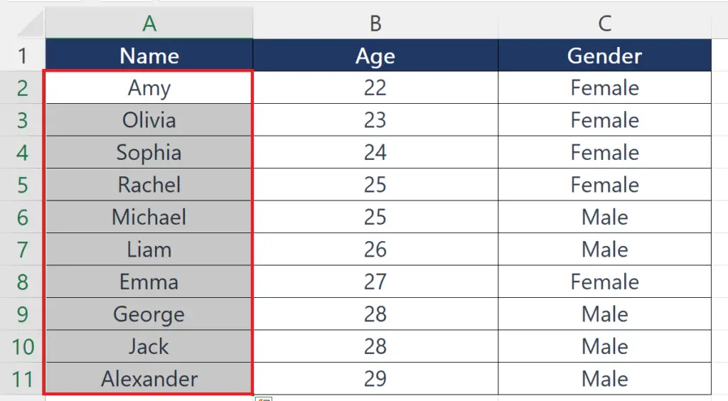
• Select the second column on the basis of which you want to sort the data.

Step 5 – Locate the “Sort & Filter” Button

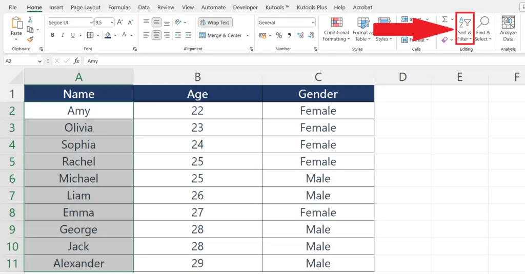
• Locate the “Sort & Filter” button in the Home tab.

Step 6 – Perform a Click on the “Sort largest to smallest” Option

• Perform a click on the “Sort largest to smallest” in the drop-down menu.
• Choose the “Expand the Selection” option in the dialog that appears and click on OK.