How to bold in Microsoft Excel

To bold in Microsoft Excel means to apply bold formatting to text in a cell or range of cells in a spreadsheet. Bolding makes the selected text appear thicker and darker than non-bolded text and is often used to emphasize important information, headings, or labels in a spreadsheet.

In this tutorial, we will learn how to bold in Microsoft Excel. In Microsoft Excel to bold is a simple task that can be achieved by utilizing the “Bold” command or the keyboard keys. Another approach to bold is by utilizing Conditional Formatting.

As an example, we want to apply bold formatting to the column in the current data set that contains the names of vehicle manufacturers.

Method 1: Utilizing the Bold Command

Step 1 – Choose the Range of Cells

• Choose the range of cells you want to bold.

Step 2 – Locate the Bold Command

• Locate and utilize the “Bold” command in the Font section located in the Home tab.

Method 2: Utilizing the Keyboard Shortcut Keys

Step 1 – Choose the Range of Cells

• Choose the range of cells you want to bold.

Step 2 – Press the CTRL+B Keys

• Press the CTRL+B keys on the keyboard.

Method 3: Utilizing the Conditional Formatting

Step 1 – Choose the Range of Cells

• Choose the range of cells you want to bold.

Step 2 – Locate the Conditional Formatting Button

• Locate the Conditional Formatting button in the Home tab.

Step 3 – Choose the “New Rule” Option

• Choose the “New Rule” option.

Step 4 – Choose the “Format only cells that contain” Option

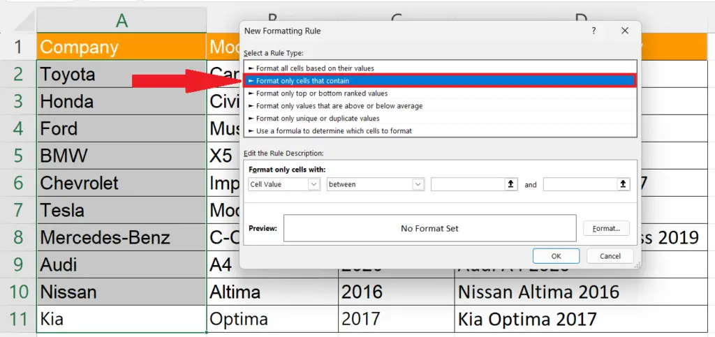
• Choose the option labeled “Format only cells that contain” option.

Step 5 – Choose the “No Blanks” Option

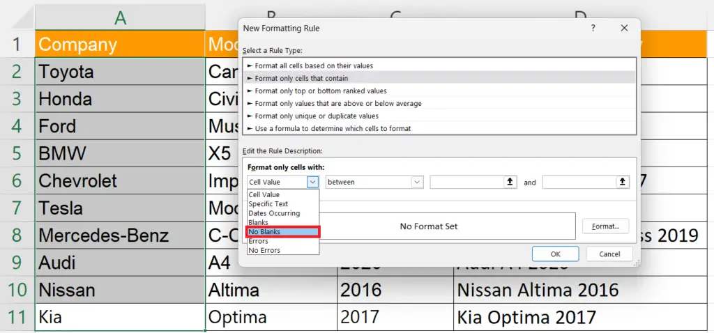
• Choose the “No Blanks” option in the  “Format only cells that with” drop-down menu.

Step 6 – Apply the Bold Format

• Perform a click on the Format button.
• Navigate to the Font tab.
• Select “Bold” as the Font Style.
• Click on OK in the “Format Cells” dialog box and the “New Formatting Rule” dialog box.