
How to average letter grades in Excel
 By
SpreadCheaters
By
SpreadCheaters
You can watch a video tutorial here.
Excel is widely used for calculations due to the several arithmetic operators and functions that it has. When trying to find the average of values that are not numerical, you need a numerical reference for each value. If you need to average letter grades, you need to first find the average of the numerical references and then get the corresponding letter grade. To do this in Excel, there are two approaches, One uses the AVERAGE() and nested IF() functions, and the second uses the AVERAGE() and IFS() functions.
- AVERAGE() function: this finds the arithmetic mean of a set of numbers
- Syntax: AVERAGE(range of numbers)
- range of numbers: if there is only a single number, then it cannot return the average
- Syntax: AVERAGE(range of numbers)
- IF() function: this evaluates a condition and returns one value if true and another if false.
- Syntax: IF(logical test, value if true, value if false)
- logical test: this is any condition that will result in either a true or false value
- value if true: this can be any type of data that will be displayed if the logical test evaluates to true
- value if false: this can be any type of data that will be displayed if the logical test evaluates to false
- Syntax: IF(logical test, value if true, value if false)
A nested IF() function combines many IF() functions into one. Let’s break it up to see how it works:
IF(logical test1, value if logical test1 is true,
IF(logical test2, value if logical test2 is true,
IF(logical test3, value if logical test3 is true,
value if all logical tests are false)))
In each IF statement, instead of the value for the false result, another IF statement is inserted. It is like saying “In case this test fails, try this next test”. This continues until all the tests have been completed and then the final value for the false result is stated in case all tests evaluate to false.
- IFS() function: this evaluates multiple conditions and returns the first value that evaluates to true
- Syntax: IFS(logical test1, value if logical test1 is true, logical test2, value if logical test2 is true……)
- logical test: this is any condition that will result in either a true or false value
- value if true: this can be any type of data that will be displayed if the logical test evaluates to true
Option 1 – Use nested IF() functions
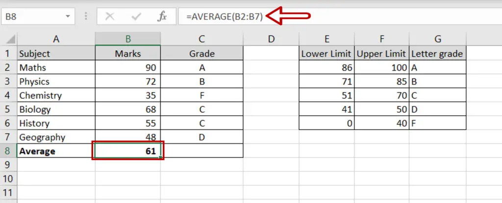
Step 1 – Use the AVERAGE() function

- Select the cell in which you want the result to appear
- Type the formula using the cell references:
= AVERAGE (Marks)
- Press Enter
Step 2 – Create the nested IF() functions
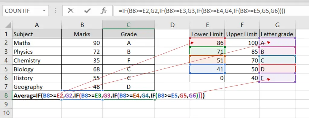
- Select the cell where the average letter grade is to appear
- Create the formula using cell references:
=IF(Average >= Lower Limit1, Letter Grade1,
IF(Average >= Lower Limit2, Letter Grade2,
IF(Average >= Lower Limit3, Letter Grade3,
IF(Average >= Lower Limit4, Letter Grade4,
Letter Grade5))))
- Press Enter
Step 3 – Check the result
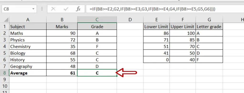
- The average grade is displayed
- If the marks or the grade scale changes, the result will be updated automatically
Option 2 – Use the IFS() function
Step 1 – Use the AVERAGE() function
- Select the cell in which you want the result to appear
- Type the formula using the cell references:
= AVERAGE (Marks)
- Press Enter
Step 2 – Create the formula
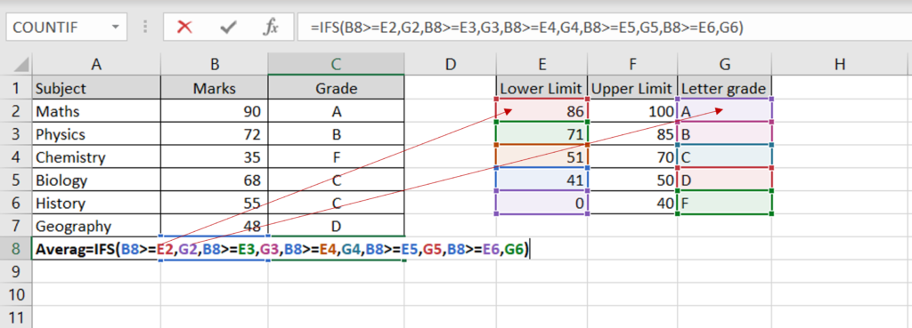
- Select the cell where the average letter grade is to appear
- Create the formula using cell references:
=IFS(Average >= Lower Limit1, Letter Grade1,
Average >= Lower Limit2, Letter Grade2,
Average >= Lower Limit3, Letter Grade3,
Average >= Lower Limit4, Letter Grade4,
Average >= Lower Limit5, Letter Grade5)
- Press Enter
Note: The order in which the tests are given is very important because the function returns the value for the first condition that tests true. In this case, if the conditions are given in ascending order i.e. starting from >=0, the first condition will evaluate true and ‘F’ will be displayed.
Step 3 – Check the result
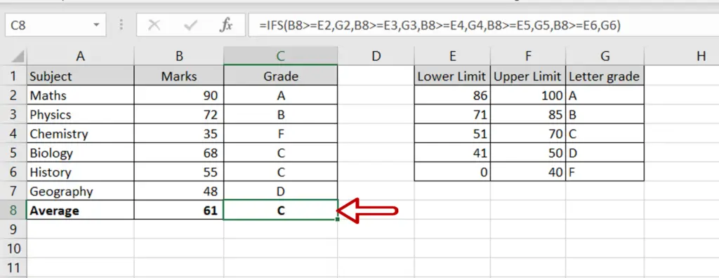
- The average grade is displayed
- If the marks or the grade scale changes, the result will be updated automatically


