
How to auto-number in Microsoft Excel
 By
SpreadCheaters
By
SpreadCheaters
The auto-numbering in Microsoft Excel is a useful process that can help streamline your data management process. With this feature, you can easily reference and organize your data, even if your data tables don’t start at the top of your spreadsheet. By automatically generating unique numbers for each row in your data, you can quickly and easily identify and track specific rows, without the need to manually enter row numbers.
In this tutorial, we will learn how to auto-number a range in Microsoft Excel. In Excel, numbers can be added to a data set in various methods. We can use the Autofill feature to add the numbers, we can use the ROW function to add numbers. Alternatively, the SEQUENCE function can also be utilized.
For instance, we will add serial numbers in a column by auto-numbering. For this, we will use the above mentioned methods.
Method 1: Auto-Number using the ROW Function
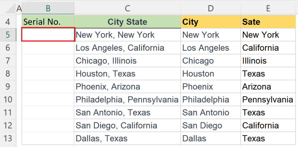
Step 1 – Select a Blank Cell
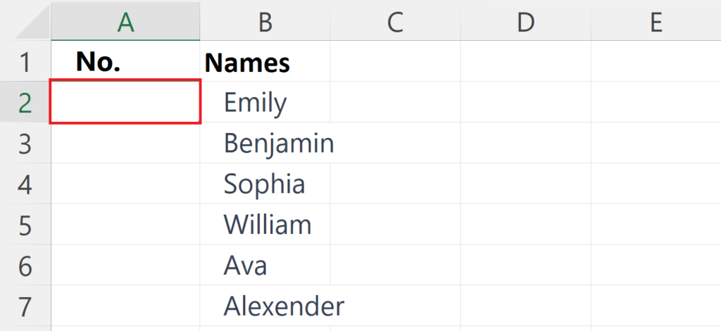
- Select a blank cell.
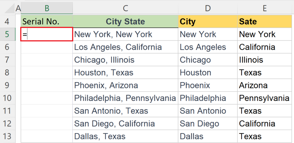
Step 2 – Place an Equals Sign
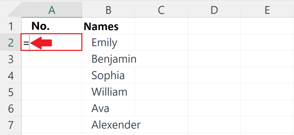
- Place an Equals sign in the blank cell.
Step 3 – Enter the ROW Function
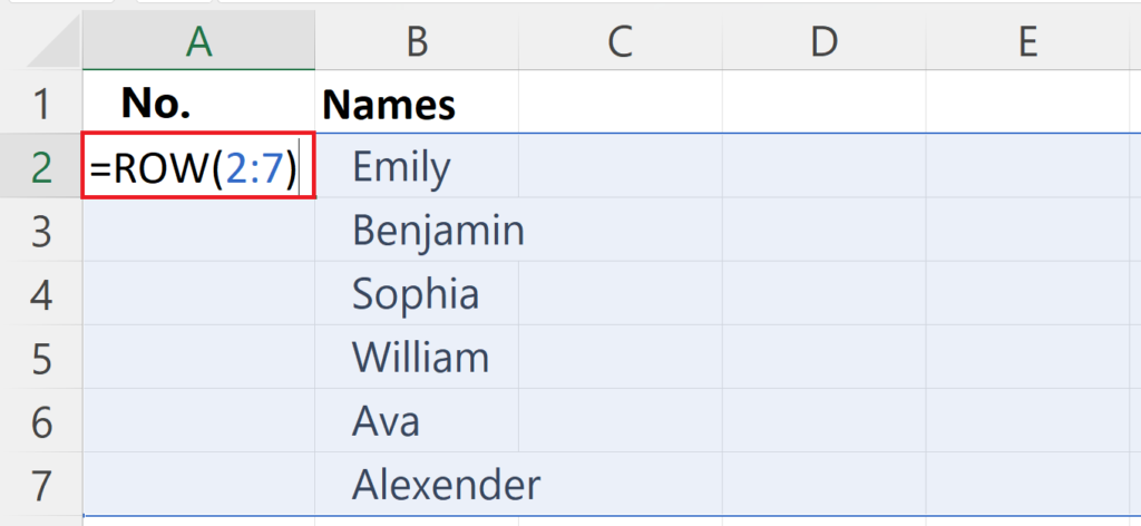
- The syntax of the ROW function is:
ROW(2:7)
- Where the first argument is the number from which you want to start the list.
- The second argument is the number where the list has to end.
Step 4 – Press the Enter Key
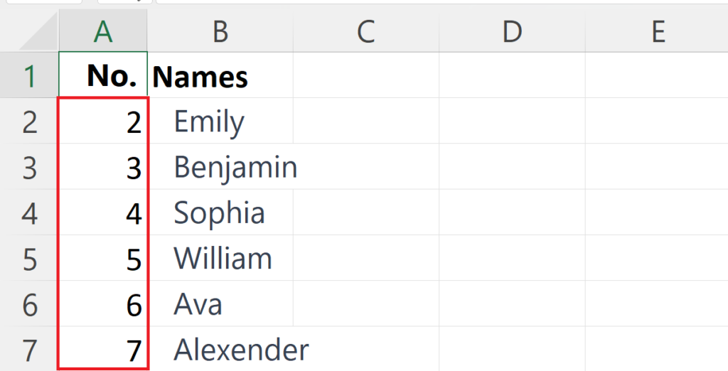
- Press the Enter key.
Method 2: Auto-Number using the SEQUENCE Function
Step 1 – Select a Blank Cell
- Select a blank cell.
Step 2 – Place an Equals Sign
- Place an Equals sign in the blank cell.
Step 3 – Enter the SEQUENCE Function
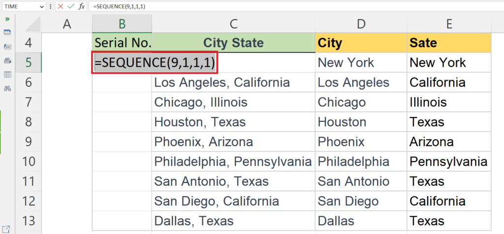
- The syntax of the SEQUENCE function is:
SEQUENCE(9,1,1,1)
- The first argument 9 is the number of rows and the second argument is the number of columns.
- The third and fourth arguments are the starting and the step of the sequence, respectively.
Step 4 – Press the Enter Key
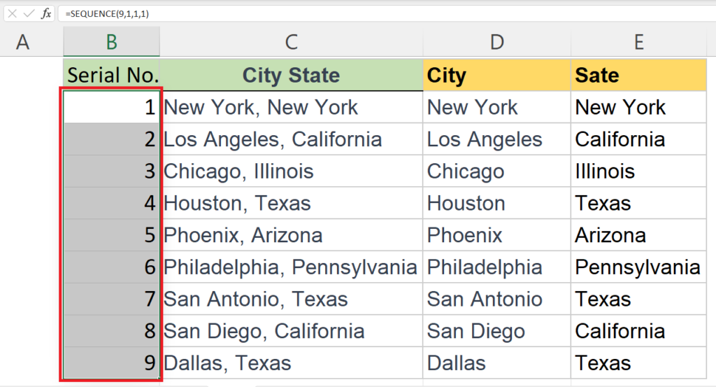
- Press the Enter key.
Method 3: Auto-Number using the Autofill Feature
Step 1 – Add the Number 1 in the First Cell
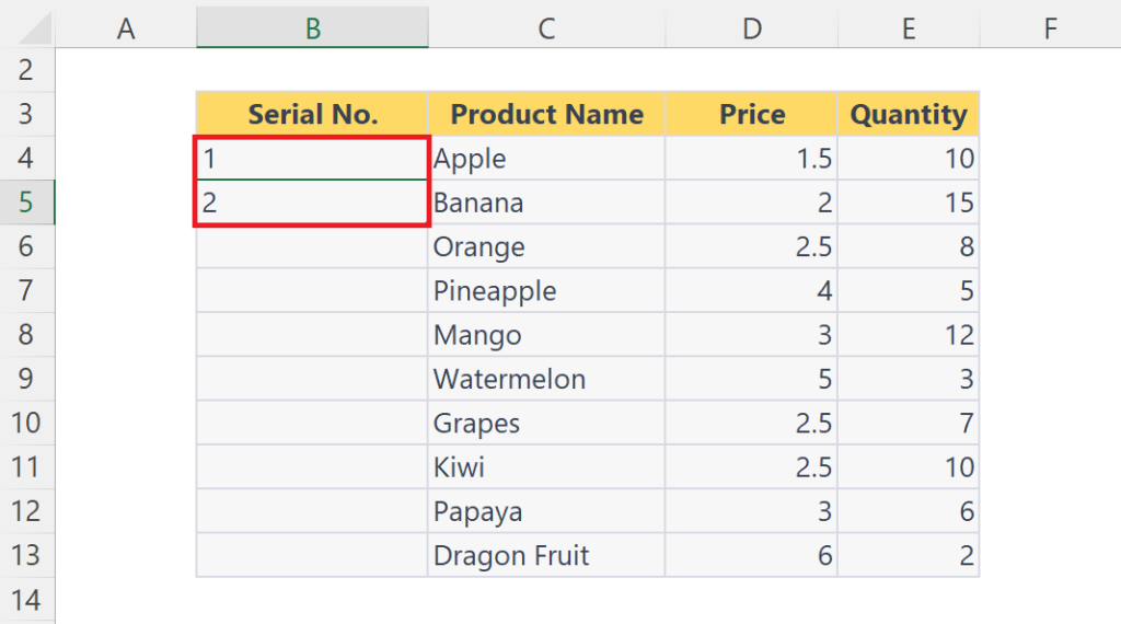
- Add the first two numbers manually in the first and second cells of the column.
Step 2 – Select the Cells
- Select the cells in which you have entered the numbers.
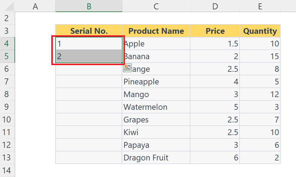
Step 3 – Hover the Cursor to the Right Bottom of the Cells
- Hover the cursor to the bottom right of the cells in which you have entered the number 1 and 2.
- The cursor will convert into a black plus sign.
Step 4 – Hold and Drag the Cursor Down, and Drop
- Hold and drag the cursor down over the cells.
- Drop the cursor.
- Numbers will be added automatically in the column.


