How to auto-number cells in Excel

You can watch a video tutorial here.

Excel has many tools and shortcuts that can be used to automate repetitive tasks or tasks that span a large number of rows and columns. One such task is numbering cells in a column or row. Not only is this a time-consuming task if done by typing the number in each cell, but the possibility of errors is high. Here we will look at different ways of auto-numbering the cells in Excel:

1. Fill handle: this uses the fill tool from the cells
2. Fill menu option: this uses the fill tool from the ribbon 
3. ROW() function: this returns the row number of the cell reference
   1. Syntax: ROW(cell reference)
      1. cell reference: the reference of the cell for which you want the row number. If this is left blank, it takes the row number of the cell it is in
4. SEQUENCE() function: this generates a matrix of numbers according
   1. Syntax: SEQUENCE(rows, columns, start, step)
      1. rows: the number of rows in the matrix
      2. columns: the number of columns in the matrix
      3. start: the start number
      4. step: the number by which each number should increment

Note: These same methods can be used to generate numbers across rows.

Option 1 – Use the fill handle

Step 1 – Type the numbers

• In the first two rows of the column where the series is to be filled, type the first two numbers of the sequence i.e. 1,2

Step 2 – Use the fill handle

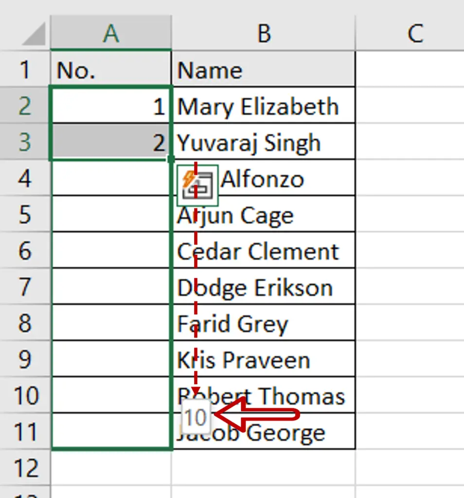
• Select the rows and use the fill handle at the lower right corner of the second cell to drag the box down
• The sequence of numbers being generated will be displayed as you drag the handle down
• Release the handle when you reach the last number 

Option 2 – Use the fill menu option

Step 1 – Type the first number

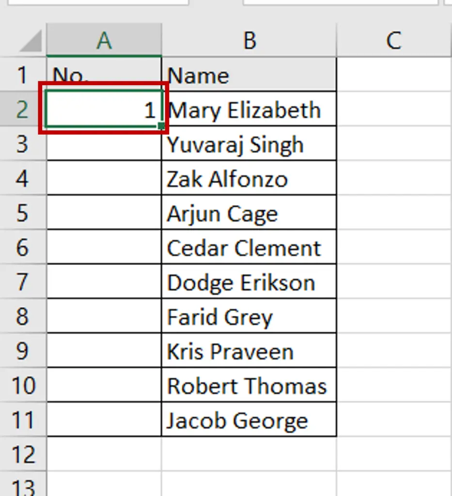
• In the first row of the column in which the numbers are to be filled, type the first number i.e. 1

Step 2 – Open the Series box

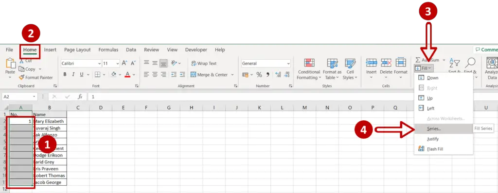
• Select the column where the series is to be filled
• Go to Home > Editing and click the Fill button
• Select Series from the drop-down menu

Step 3 – Set the parameters

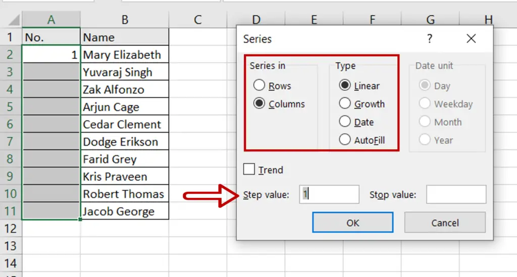
• In the Series box, set the following:
  • Series in: Columns
  • Type: Linear
  • Step value: 1
• Click OK

Step 4 – Check the result

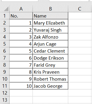
• The list of numbers is created

Option 3 – Use the ROW() function

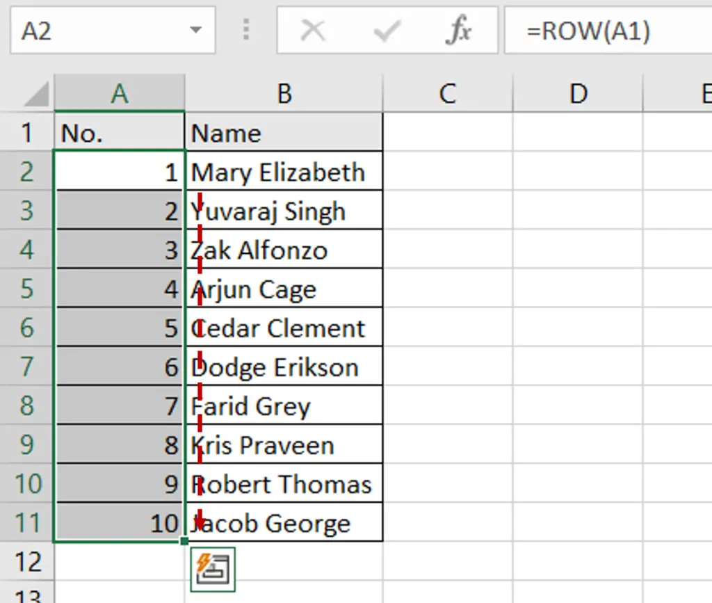
Step 1 – Type the formula

• Select the first cell of the column where the series is to be filled
• Type the formula:

=ROW(cell reference of the previous row)

• Press Enter

Step 2 – Copy the formula

• Using the fill handle from the first cell, drag the formula to the remaining cells

OR

1. Select the cell with the formula and press Ctrl+C or choose Copy from the context menu (right-click)
2. Select the rest of the cells in the column and press Ctrl+V or choose Paste from the context menu (right-click)

Step 3 – Check the result

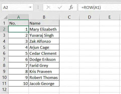
• The list of numbers is created

Option 4 – Use the SEQUENCE() function

Step 1 – Type the formula

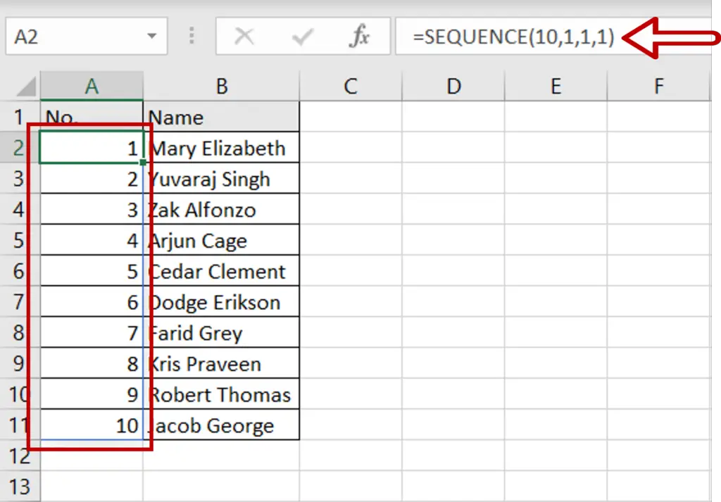
• In the first cell of the column where the series is to be filled, type:

=SEQUENCE(10,1,1,1)

• This is for 10 rows, 1 column, starting at 1 and incrementing by 1
• Press Enter
• The sequence of numbers is created