
How to assign Letter Grades in Excel
 By
SpreadCheaters
By
SpreadCheaters
Grading is an essential part of academic life, and it is crucial to be able to assign grades accurately and efficiently. Microsoft Excel can make the Grading process more efficient, accurate, and organized. In this tutorial, we will assign letter grades in Excel.
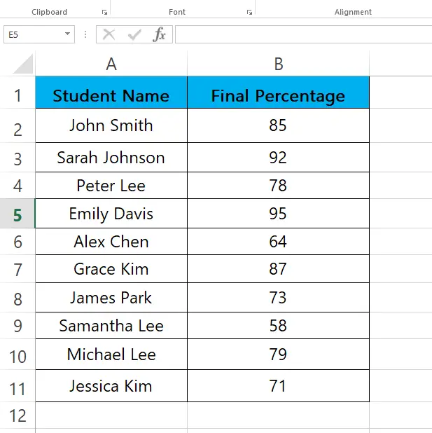
Here we have a dataset that contains Student Names, and their Final Percentage. In the tutorial we will learn how to assign Letter Grades to the students according to their Final Percentage, Grading System is also given for reference. Let’s look at the dataset.
Method – 1 Using the IF formula.
Step – 1 Type the formula.
- Select the cell where you want the result.
- The generic formula for our case will be as follows;
=IF(Cell_address 1st_Condition,”Result“,IF(Cell_address 2nd_Condition,”Result“,IF(Cell_address 3rd_Condition,”Result“,IF(Cell_address 4th_Condition,”Result“,” Result_if _no_condition_matches “))))
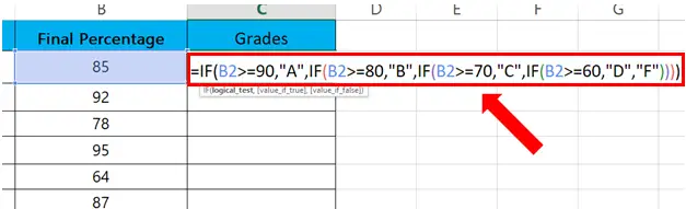
- The actual formula will be;
=IF(A2>=90,”A”,IF(A2>=80,”B”,IF(A2>=70,”C”,IF(A2>=60,”D”,”F”))))
The formula explanation is given at the end of the document.
- Press enter to implement the formula in the first cell.
Step – 2 Find values for the rest of the cells.
- Select the cell where you have implemented the formula in last step.
- Drag the cell from the bottom right to the rest of the cells.
- Grades will appear automatically.
Method – 2 Using VLOOKUP.
Step – 1 Create the LOOKUP Table
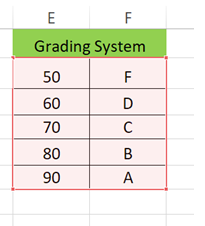
- Lookup table is really important as it defines the rules for grading. Address of the lookup table is used in the VLOOKUP formula for grading.
- To add the LOOKUP table select a cell and enter a number in one cell and the corresponding grade to the cell beside it, in our case in the cell E2 we added the number and in F2 we added the corresponding grade.
- Repeat the above steps for the rest of the cells in the column for the LOOKUP table.
- LOOKUP table is shown above.
Step – 2 Type the formula.
- Select the appropriate cell.
- Syntax of the formula is:
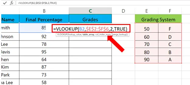
=VLOOKUP(Student_percentage_Cell_address, Range_of_cells_to_lookup, column_number_of_lookup_table ,True)
- In our case the formula will be
=VLOOKUP(B3,$E$2:$F$6,2,TRUE)
The formula explanation is given in the last part of the document.
Step – 3 Find values for the rest of the cells.
- Select the cell with formula.
- Drag the cell from the bottom right to the rest of the cells.
- Grades will appear automatically.
Method – 3 Assigning Pass and Fail
Step – 1 Type the formula.
- Select the cell where you want the result.
- Syntax of the formula is:
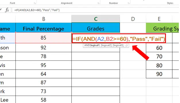
=IF(AND(Cell_Address, Cell_Address Condition),”Pass”,”Fail”)
- In our case the formula will be
=IF(AND(B5,C5>=60),”Pass”,”Fail”)
The formula explanation is given at the end of the document.
Step – 2 Find values for the rest of the cells.
- Select the cell with the formula.
- Drag the cell from the bottom right to the rest of the cells.
- Grades will appear automatically.
Formula Explanations.
Formula – 1
=IF(A2>=90,”A”,IF(A2>=80,”B”,IF(A2>=70,”C”,IF(A2>=60,”D”,”F”))))
Here, A2 is the cell containing the numerical score for the first student, and the formula will check if the score is greater than or equal to 90, if yes, then the student will be assigned an “A” grade. Otherwise, it will check the next condition (score >= 80) and give the letter grade accordingly. The process will continue until a grade is assigned based on the given scale.
Formula – 2
=VLOOKUP(B3,$E$2:$F$6,2,TRUE)
B3 is the value to look up in the first column of the table. $E$2:$F$6 is the range of the table. Note that the dollar signs ($) are used to lock the range so that it doesn’t change when we copy the formula to other cells. 2 specifies the column number in the table that contains the data we want to retrieve. TRUE is used to find an approximate match to the lookup value in the first column of the table. If a perfect match is not found, VLOOKUP will return the closest match that is less than or equal to the lookup value.
Formula – 3
=IF(AND(B5,C5>=60),”Pass”,”Fail”)
AND(B5, C5>=60) checks if both B5 and C5 are greater than or equal to 60. If both conditions are True, AND function will return TRUE, which triggers the IF function to return “Pass“. If either condition is not true, AND function will return FALSE, and the IF function returns “Fail“.


