How to assign a value to a word in Excel

In Excel, assigning a value to a word typically refers to associating a numeric value with a specific word or text string using a formula or a lookup function. This process is often used in data analysis or creating calculations based on specific conditions.

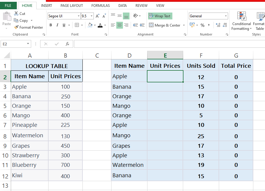
In this tutorial, we will learn how to assign a value to a word. Consider the following steps to learn this. The following dataset represents the names of the items and their prices. We will use the lookup table as the reference table, this reference table has the item names and unit prices assigned to them, this will be used for assigning the value to a word in the next table. The advantage of having a lookup table to assign unit prices is that we will have to change the unit prices only once in the table and all formulas will be updated accordingly.

Method 1 – Assigning a value to a word by using VLOOKUP

In this method, we will discuss how to assign a value to a word using VLOOKUP Function in Excel. Follow the given steps to learn how to achieve this. The Syntax of the VLOOKUP formula is as follows;

=VLOOKUP(lookup_value, table_array, col_index_num, range_lookup)

Follow the link above to learn more about the syntax of VLOOKUP.

Step 1 – Select the cell

• Select the first cell where you want the VLOOKUP function to be applied, in our case, it will be E2.

Step 2 – Writing the formula

• Now write the formula, in our case, it will be =VLOOKUP(D2, A3:B12, 2)
• You should use the $ sign before and after the cell references to lock them so that our formula doesn’t change. 
• Now our formula will look like this: =VLOOKUP(D2, $A$3:B$12, 2). 

In this formula D2: This is the value being searched for. It represents the lookup value that you want to find in the first column of the range.

$A$3:B$12: This is the range being searched. It represents the reference table where the lookup value will be searched in. The dollar signs ($) before the column and row references make them absolute references, which means that the range will remain fixed when the formula is copied to other cells.

2: This is the column index number. It specifies which column in the range contains the value to be returned. In this case, it is 2, indicating that the value to be returned is in the second column of the range.

• Press Enter.

Step 3 – Applying it to all the cells

• If you want to apply this formula to all the cells, drag it down using a fill handle.
• Column G represents the total price, it will multiply the unit price by the unit sold by using a formula that is: =E2*F2. 

Method 2 – Assigning a value to a word by using XLOOKUP

In this method, we will learn how to assign a value to a word by using the XLOOKUP function in Excel. The XLOOKUP function in Excel allows you to perform advanced lookups, including searching for values in both vertical and horizontal directions. The syntax for the XLOOKUP function is as follows:

=XLOOKUP(lookup_value, lookup_array, return_array, [match_mode], [search_mode], [if_not_found]) 

lookup_value: This is the value you want to find in the lookup_array.

lookup_array: This is the range or array where you want to search for the lookup_value.

return_array: This is the range or array from which you want to retrieve the corresponding value. The return_array should have the same number of rows or columns as the lookup_array.

[if_not_found] (optional): This is the value that will be returned if the lookup_value is not found in the lookup_array. If omitted, it will default to #N/A.

[match_mode] (optional): This argument specifies the type of match to be performed. It can take the following values:

0 or 1: Exact match (default).

-1 or -2: Exact match or next smaller item.

2: Wildcard match.

-3: Next larger item.

[search_mode] (optional): This argument specifies the direction of the search. It can take the following values:

1 or TRUE: Search from top to bottom (default).

-1 or FALSE: Search from the bottom to the top.

Note: The square brackets in the syntax indicate optional arguments.

Step 1 – Select the cell.

• Select the cell where you want the results to appear.
• In our case we are selecting E2.

Step 2 – Writing the formula

• Now write the formula in our case it will be: =XLOOKUP(D2, A3:A12, B3:B12).
• You can use the $ sign before and after the cell references to lock them so that our formula doesn’t change. 
• Now our formula will look something like this: 

=XLOOKUP(D2, $A$3:$A$12, $B$3:$B$12).

• Press Enter.

In this formula, D2 is the lookup_value. It is the cell or value that you want to search for in the lookup_array.

• $A$3:$A$12 is the lookup_array. It is the range of cells or columns where you want to search for the lookup_value. In this case, it is cells A3 to A12.
• $B$3:$B$12 is the return_array. It is the range of cells or columns from which you want to retrieve the corresponding value when the lookup_value is found in the lookup_array. In this case, it is cells B3 to B12.

Step 3 – Apply the formula to all the cells

• If you want to apply the formula to all the cells, drag it down using a fill handle.
• Column G represents the total price, it will multiply the unit price by the unit sold by using a formula that is: =E2*F2,(this is optional)