
How to apply Gradient Fill in Microsoft Excel
 By
SpreadCheaters
By
SpreadCheaters
In this tutorial we will learn how to apply color gradients in Microsoft Excel. Gradient Fill is a feature in Microsoft Excel that allows users to apply a color effect to cells, shapes, or charts by transitioning smoothly between two or more colors.
Microsoft Excel is a spreadsheet software developed by Microsoft that allows users to store, organize, and analyze data. It provides features like cell formatting, conditional formatting, chart creation, pivot tables, and formula calculation. Excel is widely used for various purposes, including financial analysis, project management, and data visualization. It is available as part of the Microsoft Office suite and can also be purchased as a standalone software.
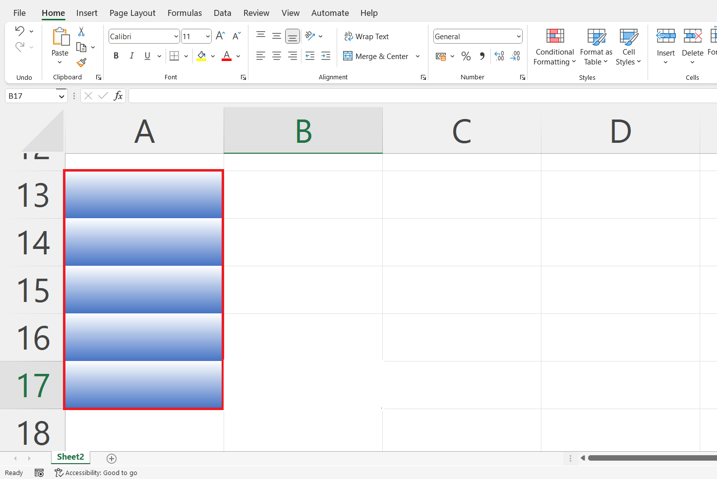
Step 1 – Select the cells
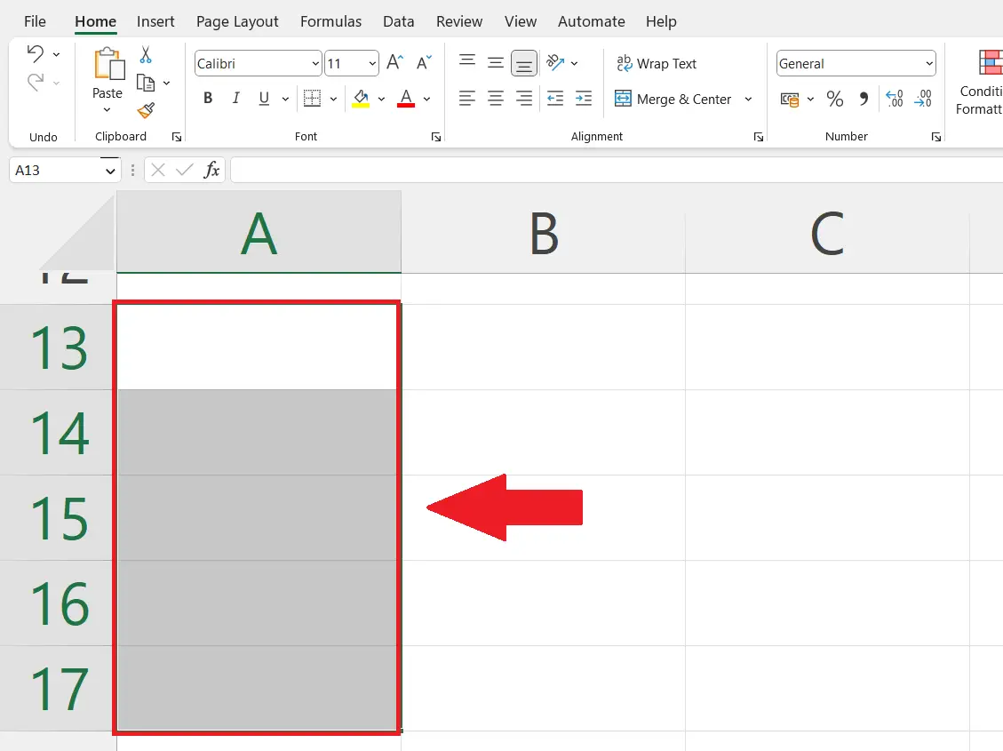
– Select the targeted cells on which you want to apply gradient fill.
Step 2 – Right Click on the cells
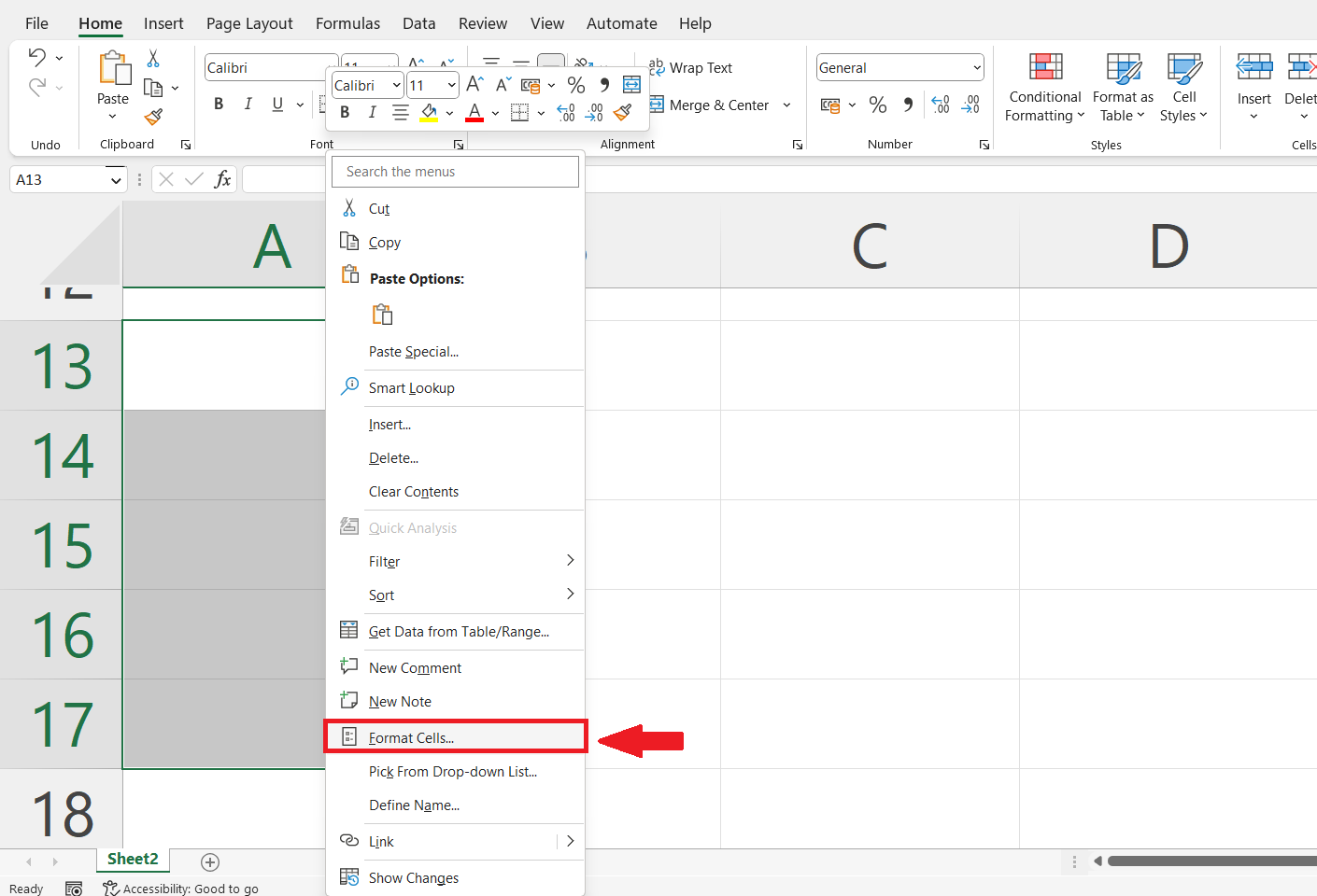
– Right click on the selected cells. A pop-up menu will appear. Click on the Format Cells option
Step 3 – Select the color
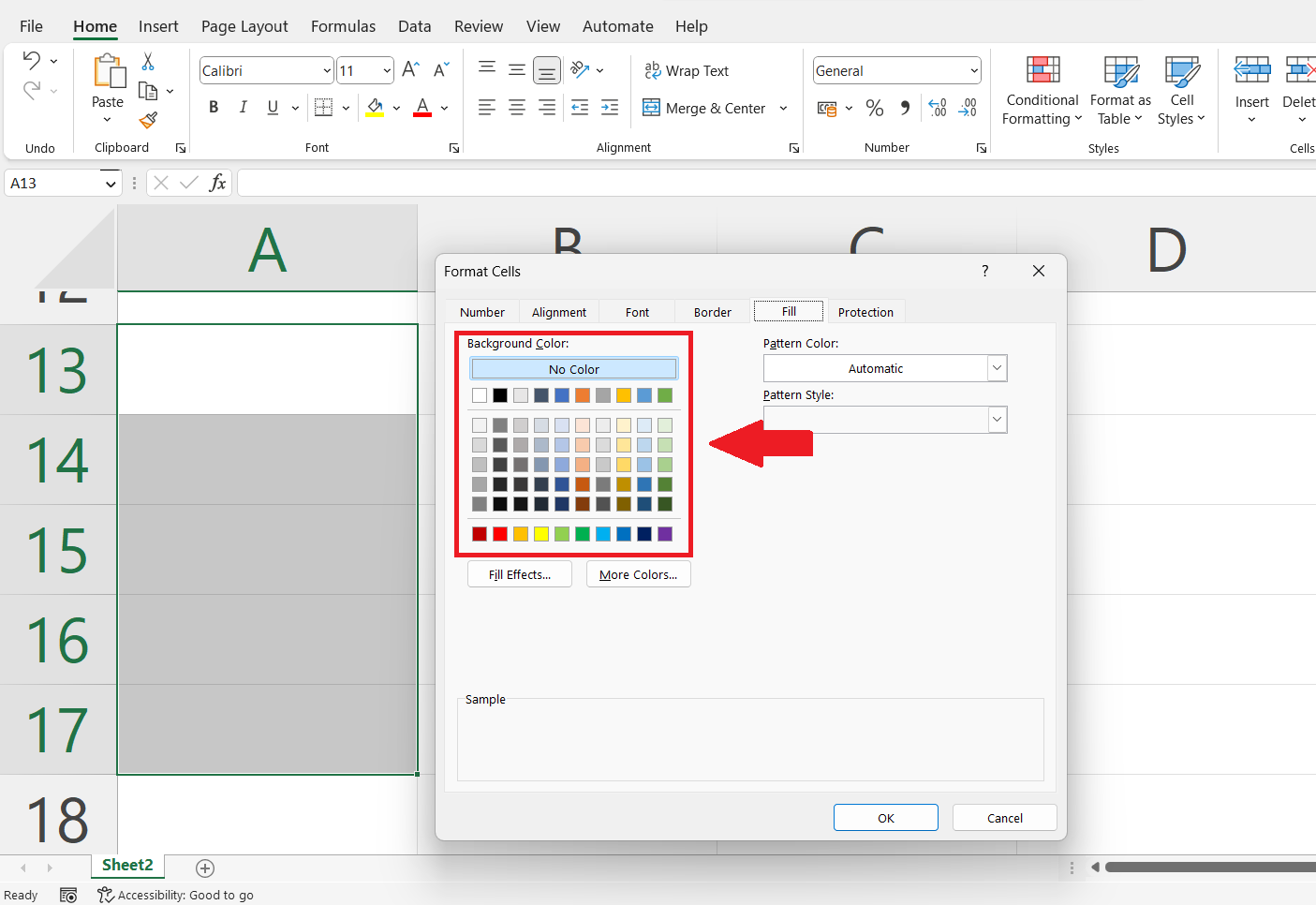
– Select the color for gradient fill in the format cells dialog box .
Step 4 – Click on the fill effects
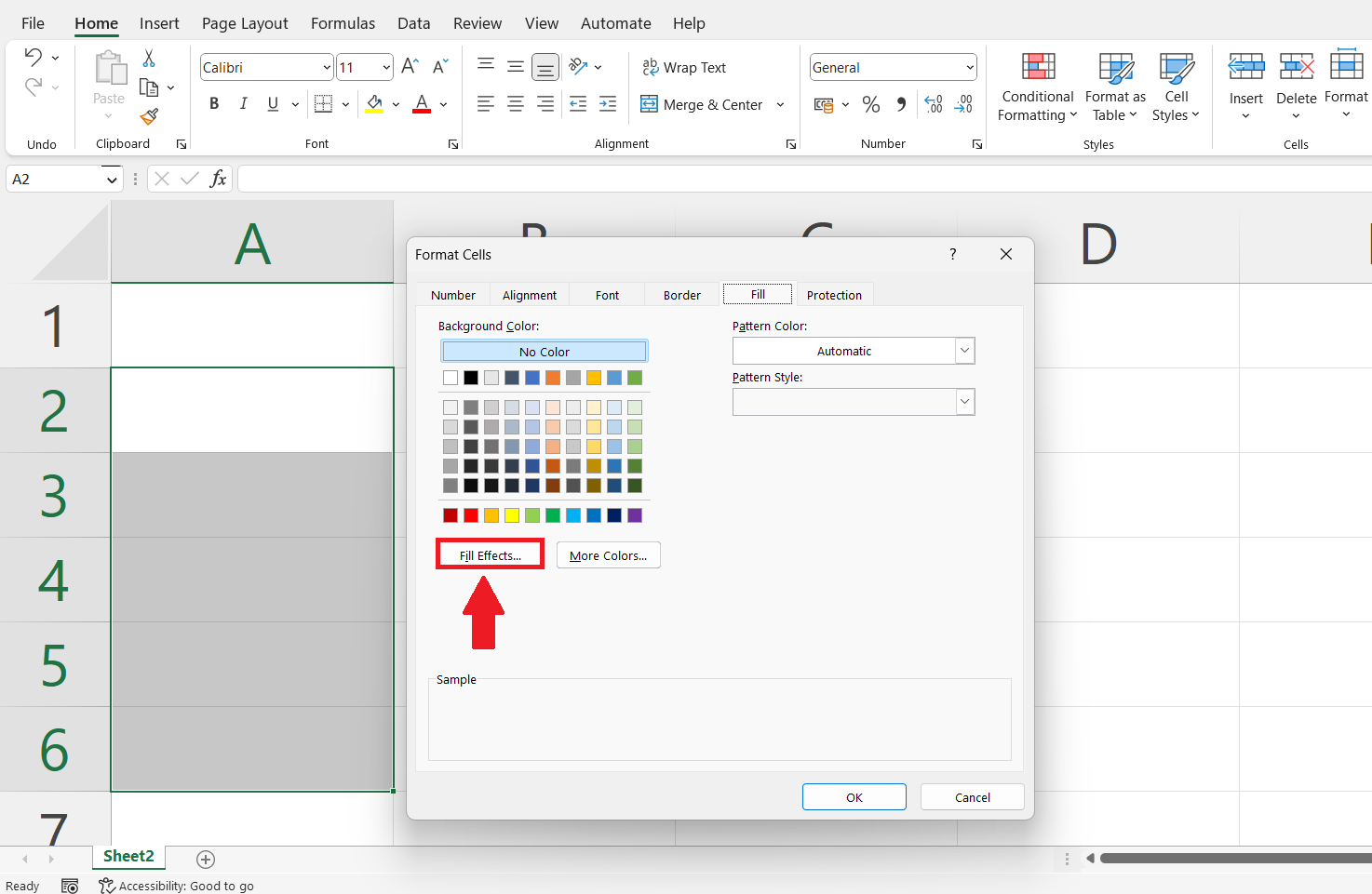
– Click on the Fill Effect option on the left-center of the format cells dialog box.
Step 5 – Select the styles of gradient fill
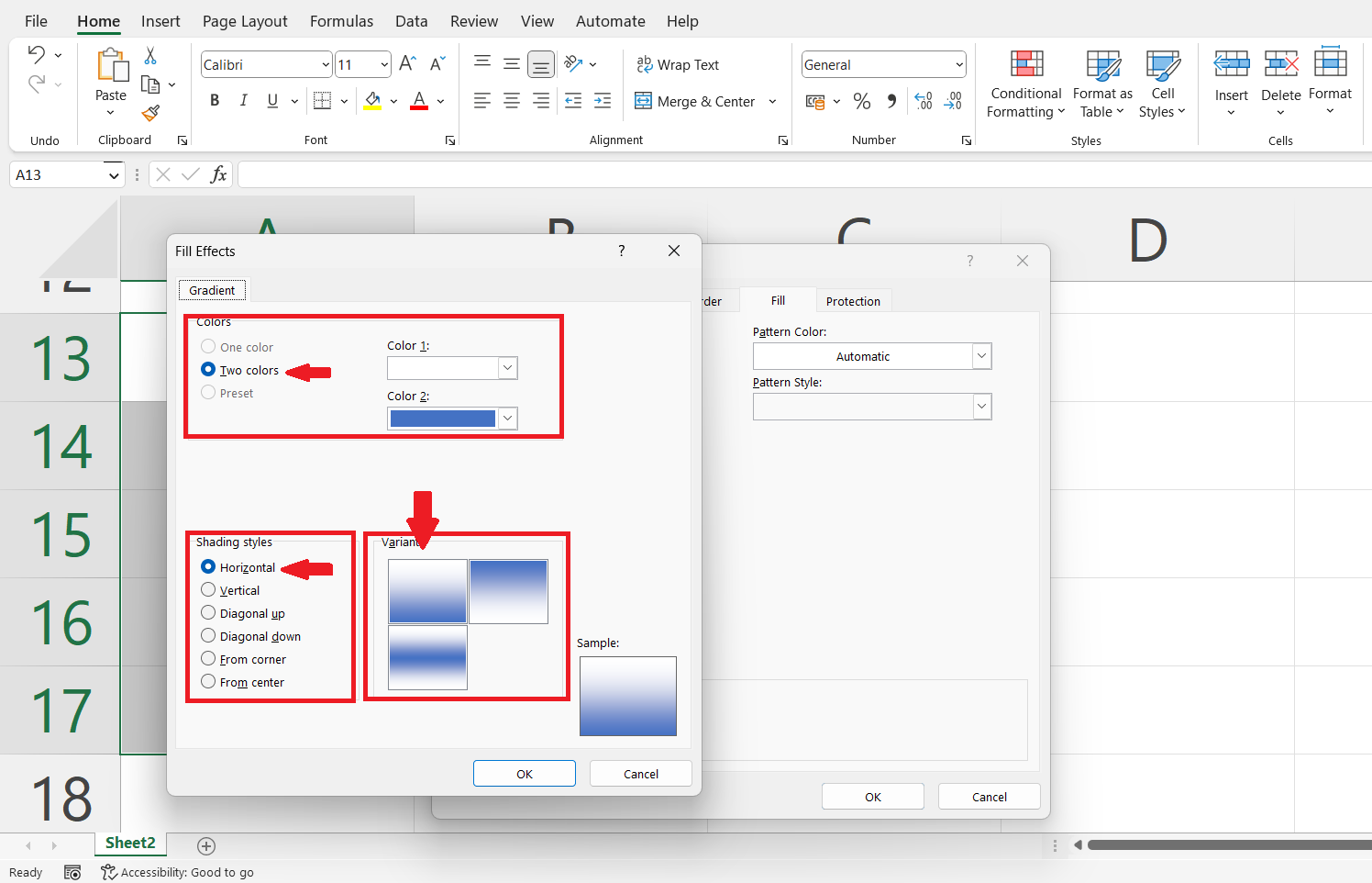
– We can select multiple colors, shading styles and the variation of the gradient fill.
Step 6 – Click on Ok
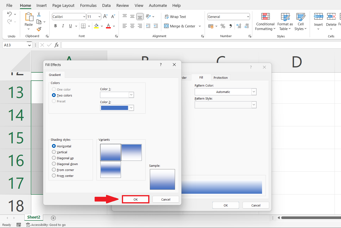
– Click on the Ok option of the Fill effects dialog box.
Step 7 – Click on Ok

– Click on the Ok option of the Format cells dialog box. Gradient fill will be applied to the targeted cells.


