How To Annualize Returns In Microsoft Excel

In this tutorial, we will learn how to annualize returns in Microsoft Excel. The annualization of returns in Excel is a commonly performed task that provides valuable insights. The general formula for annualizing returns is “((1+R)^n)-1“, with R representing the return rate and n representing the number of periods within one year.

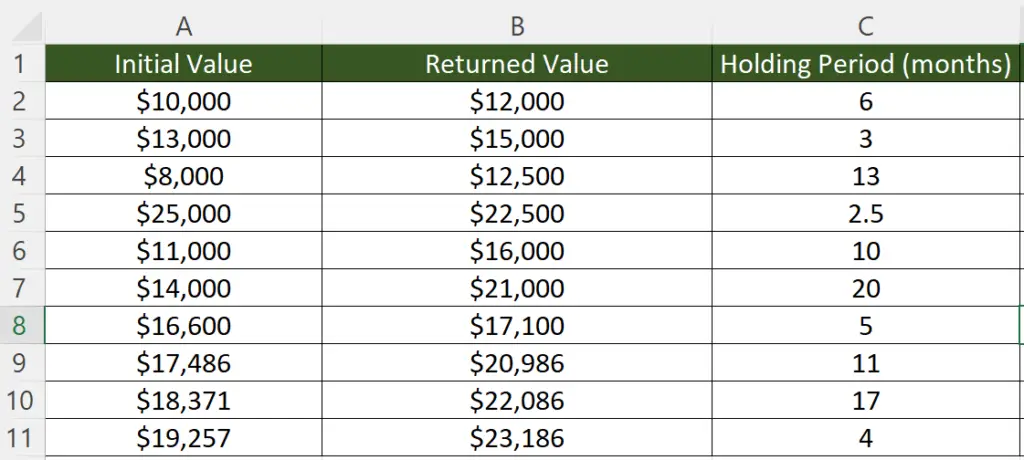
Let’s say we have a data set that represents initial values, returned values, and the holding periods for each investment. We will calculate the annualized returns for each investment utilizing the following steps.

Annualizing returns is a method that enables investors to compare the performance of various investments over diverse time frames on a yearly basis. Essentially, it offers a means of normalizing the returns of investments with varying holding periods, which aids investors in making better-informed investment decisions.

Step 1 – Choose an Empty Cell

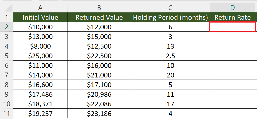
– Choose an empty cell to calculate the return percentage.

Step 2 – Calculate the Return Percentage

– Calculate the return percentage by utilizing the formula:

Step 3 – Convert the Holding Period into Years

– Choose an Empty cell.
– Convert the holding period into years i.e. in this case we have a holding period in months, we will divide it by 12 to get the holding period in years.

Step 4 – Calculate the Annualized Returns

– Calculate the annualized returns.
– The structure of the formula would be:
((1+(D2)^E2)-1)
– Where cell D2 contains the rate of return and cell F2 contains the holding period in years.