
How to add text to cell in Excel
 By
SpreadCheaters
By
SpreadCheaters
While adding text to a cell in excel might seem trivial, there are a bundle of functions in excel to work with text in different ways. Let’s find out.
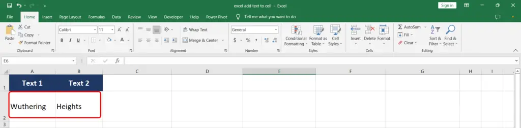
So we have a couple of cells with text in them in an excel worksheet as shown.
In this example we are going to use the following operators and functions to add text to different cells in the given worksheet.
- & Operator
- CONCATENATE
- CONCAT
- TEXTJOIN
- REPLACE
- SUBSTITUTE
Excel is a very powerful tool for data manipulation and provides many functions and tools to analyze and clean data. However, at the same time it provides a lot of other functions to work with text data. One such requirement can be adding text to a cell, which already contains text or numeric data.
Step 1 – Working with the & operator
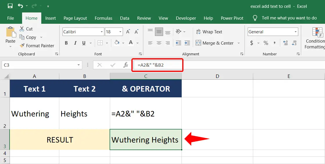
– So first of all let’s start with the ‘&’ operator also known as ampersand.
– The syntax for the formula is given below.
= text1 & text2
– Start by typing equal sign ‘=’, then click cell A2 followed by the ampersand ‘&’ operator. Then type space within quotes i.e. “ ”. Again type the ‘&’ operator and finally click the cell B2. Finally press enter.
– The cell C2 will now contain ‘Wuthering Heights’.
Step 2 – CONCATENATE function
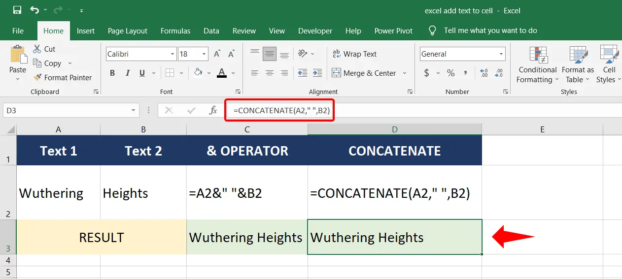
– The CONCATENATE function, now an older version of the new CONCAT function, allows text concatenation.
– The function has the following syntax,
=CONCATENATE(text1, [text2], [text3], [text4]…)
– So start by typing equal sign ‘=’ followed by the word CONCATENATE, then type open parenthesis and click the cell A2. Then type comma followed by space between quotes i.e. “ ” and then comma again. Click cell B2 and then close parentheses. Finally press enter.
– CONCATENATE does not allow range inputs.
Step 3 – CONCAT function
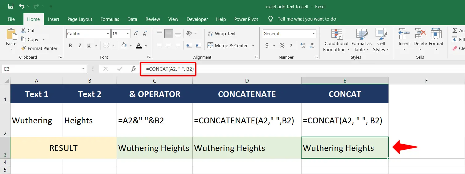
– CONCAT function is the new version of CONCATENATE.
– The CONCAT function allows range input as well.
– The syntax is similar to the CONCATENATE function.
=CONCAT(text1,…)
– So start by typing the equal sign ‘=’ followed by the word CONCAT. Then type open parentheses and click the cell A2 then type comma. Then type space between the quotes i.e. “ ” followed by another comma. Click cell B2 followed by close parenthesis. Finally press enter.
– The cell will now contain the result of the typed function as shown in the image.
Step 4 – TEXTJOIN function
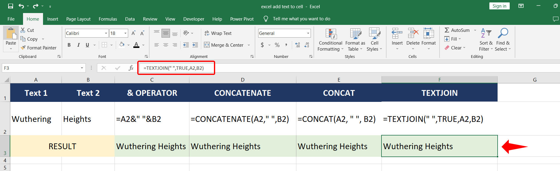
– The TEXTJOIN function has the following syntax.
=TEXTJOIN(delimiter, ignore_empty, text1, [text2], [text3], [text4], …]
– One of the two additional attributes is the delimiter allowing the joining texts to be separated by a given delimiter such as space or -.
– The second attribute is an option to ignore the empty inputs or include them. It can have a TRUE or FALSE value.
– So type the following formula in the cell you want.
=TEXTJOIN(“ ”, TRUE, A2, B2)
– We can use the range input for contiguous data in the form A2:B2. We can also use a combination of ranges and independent cells and text values.
– Pressing enter will place the result of the formula in the selected cell.
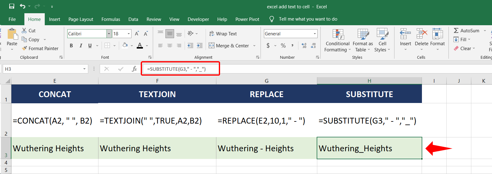
Step 5 – REPLACE function
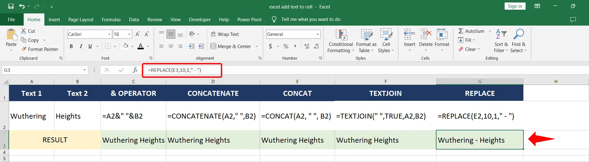
– The REPLACE function allows replacing a specific number of characters within a text with some other text as desired.
– In this example we are going to replace the space between the words in the result of the CONCAT function with a dash i.e. “-” having spaces on both sides of it.
– The syntax of the replace function is,
=REPLACE(old_text, start_num, num_chars, new_text)
– The space is the 10th character in the word ‘Wuthering Heights’ and we are going to replace only the space character. So the start_num input will have 10 in it while the num_chars will be 1.
– The new_text will have a dash with spaces on both sides i.e. “ – ”.
– So start by typing equal sign ‘=’ followed by the word REPLACE and open parentheses. Click the cell E3 followed by a comma. Then write the number 10 to provide the location of space in the original text. Then type 1 to indicate that only one character is to be replaced.
– Finally provide the dash with spaces on both sides written between quotes i.e. “ – ”.
– On pressing enter the phrase ‘Wuthering – Heights’ appears in the cell as shown.
Step 6 – SUBSTITUTE function

– The last function that we are going to look at here is SUBSTITUTE.
– SUBSTITUTE provides a lot of flexibility as it allows the option to substitute at the optional instance of a particular text that you want to replace.
– The syntax of SUBSTITUTE function is,
=SUBSTITUTE(text, old_text, new_text, [instance_num])
– So start by typing =SUBSTITUTE(.
– Click the cell G3 to indicate the text we are going to modify. Then type a comma.
– Type dash with spaces on both sides between quotes i.e. “ – ” followed by a comma.
– Type underscore between quotes as the new_text i.e. “_” followed by close parenthesis.
– Press enter and the cell will now contain the text ‘Wuthering_Heights’ as shown.
– So now we have learned 6 ways of adding text to a cell in excel.


