How to Add Subtotals to a Pivot Table in Microsoft Excel

In Microsoft Excel, subtotals in a pivot table are a way to summarize and group data based on a particular field. When you add subtotals to a pivot table, Excel will calculate and display the subtotal for each group of data that matches a specific field value.

This tutorial will teach you how to add subtotals in Microsoft Excel. There are various techniques to add subtotals in Excel, including the design tab, context menu, or field setting option.

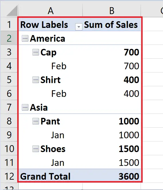
Suppose you have a sales dataset for a clothing store that sells shirts, pants, and shoes in four regions – North, South, East, and West. By using subtotals in this pivot table, you can easily see the total sales for each product and region, and identify which products and regions are generating the most revenue for the store.

Method 1: Using the Field Setting

Step 1 – Choose the Pivot Table

• Choose the pivot table in which you want to add subtotals by simply clicking on it.

Step 2 – Perform a Click on the “PivotTable Analyze” tab in the Excel Menu Bar.

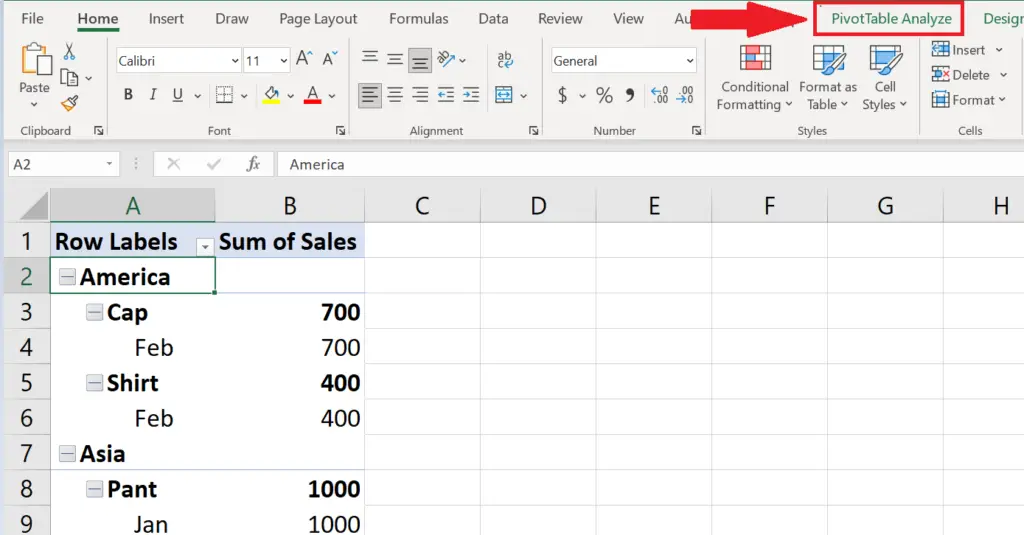
• Perform a click on the tab to access its options, including the “Field Settings” button for adding subtotals to the pivot table.

Step 3 – Perform a Click on Field Setting Option

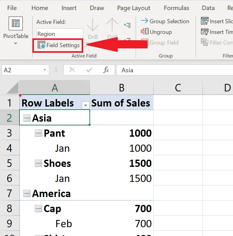
• Perform a click on the field setting option in the active field group as shown in the figure.

Step 4 – Perform a Click on the Subtotal & Filter tab

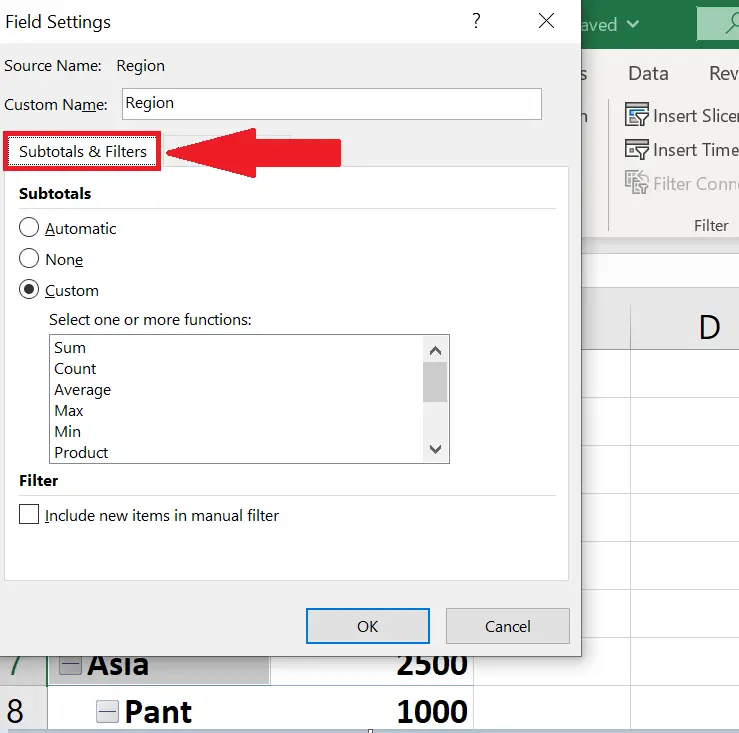
• In the “Field Settings” dialog box, click on “Subtotals & Filters”.

Step 5 – Select the Automatic Option in Subtotals section

• Under the “Subtotals” section, select the “Automatic” option or choose a specific function from the dropdown list (e.g. Sum, Average, Count, etc.) to apply to the subtotal. We will use automatic as an example here.

Step 6 – Hit the OK Button

• Hit the OK button for the addition of subtotal to the pivot table.

Method 2: Adding Subtotal to a Pivot Table in Microsoft Excel Utilizing Design Tab

Step 1 – Click Anywhere in the Pivot Table

• Perform a click inside the pivot table to activate the Design tab in the menu bar.

Step 2 – Locate the Design Tab

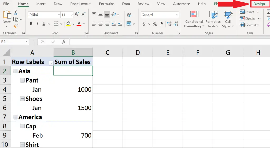
• Locate the “Design” tab in the menu bar.

Step 3 – Perform a Click on the Subtotals Button

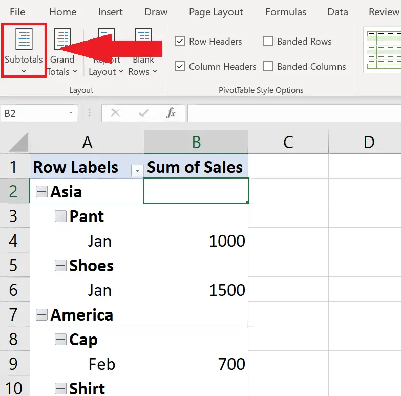
●      Perform a click on the Subtotals button on the leftmost of the ribbon.

Step 4 – Choose the Desired Subtotals Option

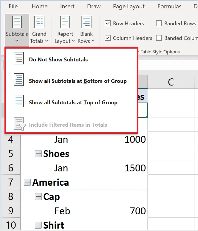
• Perform a click on the desired option from the drop-down menu.
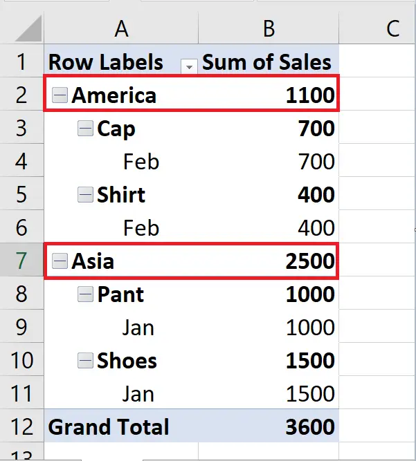
• In this case, we will utilize “Add all Subtotal at Bottom of Group”.

Step 5 – Excel will Automatically Add Subtotals to the Pivot Table

• By clicking on a selected subtotal, Microsoft Excel will automatically add it to the pivot table.