How to add significance asterisk in Microsoft Excel 

In Excel, a significance asterisk is often used to indicate the level of statistical significance of a result. This is typically represented as an asterisk (*) next to a numerical value in a table or chart. Adding a significance asterisk to your results in Excel can help to quickly and clearly communicate the level of significance to others who are viewing your data.

In this tutorial, we will learn how to add a significance asterisk in Microsoft Excel. There is no specific function or feature in Excel that automatically adds significant asterisks to your data. However, you can manually add asterisks. For this, we can use the Text Box or we can use the Data Labels built-in feature to add a significance asterisk.

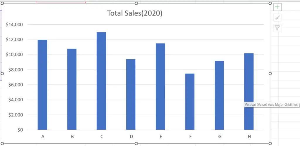
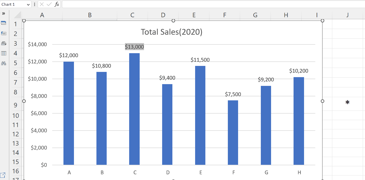
In the current data set, we have sales of some products for the year 2020. We want to add the significance asterisk to the product having the highest sales i.e. Product C.

Method 1: Adding Asterisk Using a Text Box

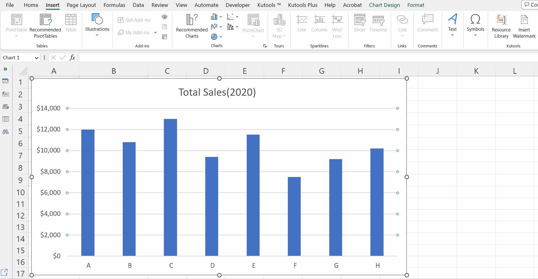
Step 1 – Go to the Insert Tab

• Go to the Insert tab in the menu bar.

Step 2 – Locate the Text Button

• Locate and click on the Text button in the Insert ribbon.

Step 3 – Click on the Text Box option

• Click on the Text Box option.
• The cursor will convert into an arrow.

Step 4 – Insert the Text Box on the Graph

• Click on the graph where you want to add the significance asterisk.
• The text box will be inserted.

Step 5 – Enter the Asterisk Mark

• Enter the asterisk mark in the text box.
• Click anywhere outside the text box to deactivate the text box.
• The significance asterisk will be added to the desired place.

Method 2: Add Asterisk using the Data Labels

Step 1 – Click on the Anywhere on the Graph

• Click anywhere on the graph.
• The “Chart Elements” plus sign will appear on the top-right corner of the graph.

Step 2 – Click on the  “Chart Elements” Plus Sign

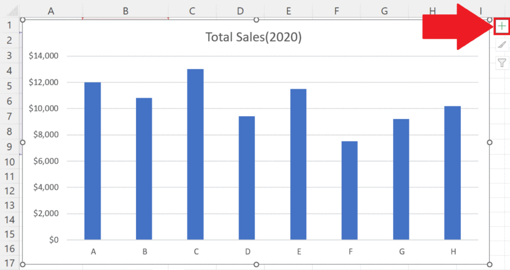
• Click on the “Chart Elements” plus sign.
• The Chart Elements list will appear.

Step 3 – Check the Box Next to the Data Elements Option 

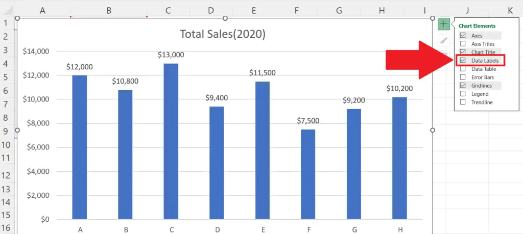
• Check the box next to the Data Elements option in the list.

Step 4 – Place an Asterisk Mark in a Cell

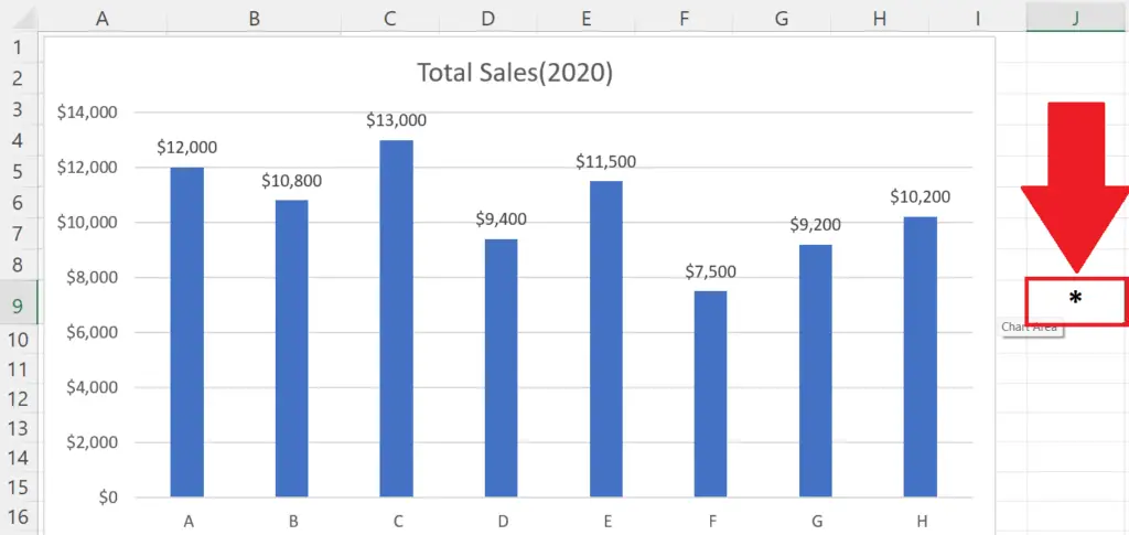
• Place an asterisk mark in a cell, we have placed an asterisk mark in cell J9.

Step 5 – Right-Click on the Data Label Click on Edit Text Option

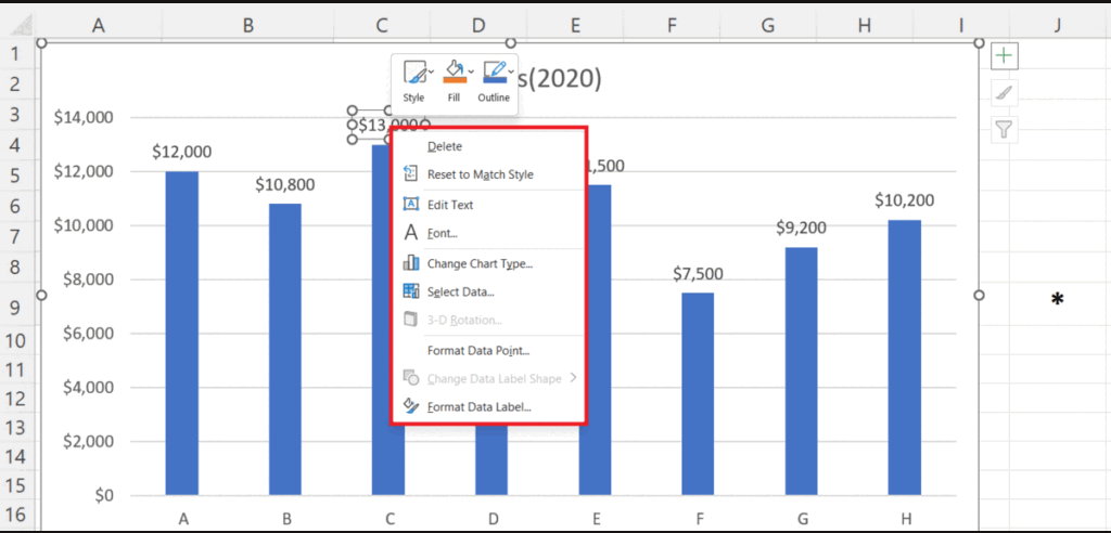
• Right-click on the Data Label to which you want to add the significance asterisk.
• A context menu will appear.
• Click on the Edit Text option in the context menu.

Step 6 – Enter the Reference of the Cell Containing the Asterisk

• Place an Equals sign in the formulae bar.
• Enter the reference of the cell in which the asterisk mark is placed.
• Press the Enter key, and the asterisk mark will be added.