How to add serial numbers in Microsoft Excel

Serial numbers in Excel are a series of unique numerical values assigned by Excel to each row in a dataset. These numbers allow users to quickly identify and track specific data points within a larger dataset. Excel can generate serial numbers automatically, or users can manually input them as needed. They are commonly used for sorting, filtering, and organizing data, making it simpler to analyze and extract valuable information.

In this tutorial, we will learn how to add serial numbers in Microsoft Excel. There are multiple ways to add serial numbers in Excel, and the process is relatively straightforward. One standard method is to utilize Excel’s “AutoFill” feature, Another option is to use the “ROW” function to create sequential numbers or users can employ algebraic formulae or text boxes to insert them. 

Method 1: Add Serial Numbers Using ROW Function

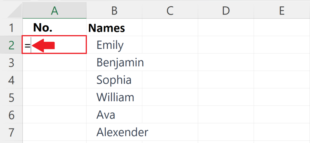
Step 1 – Select a Blank Cell

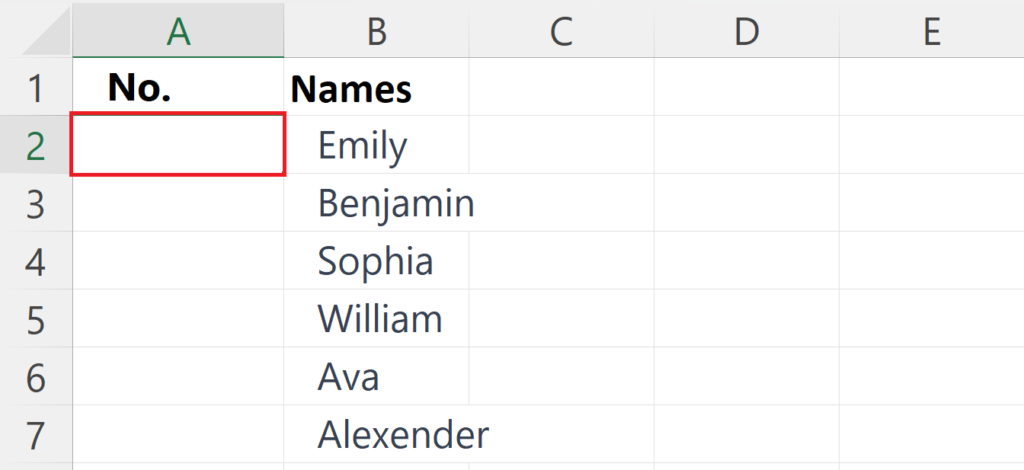
• Select a blank cell in a column in which you want to add the serial numbers.

Step 2 – Place an Equals Sign

• Place an Equals sign in the blank cell.

Step 3 – Enter the ROW Function

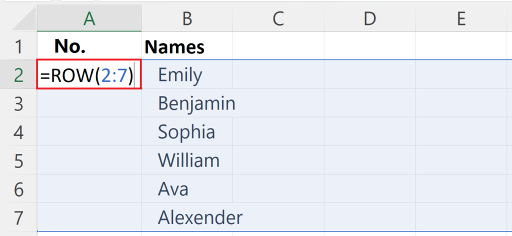
• Enter the ROW function to generate serial numbers.
• The syntax of the ROW function is: 

                                 ROW(2:7)

The ROW function accepts only one argument i.e the range of the serial numbers. For instance, we have input 2:7 as the range of serial numbers. This will generate serial numbers starting from 2 and ending at 7.

Step 4 – Press the Enter Key

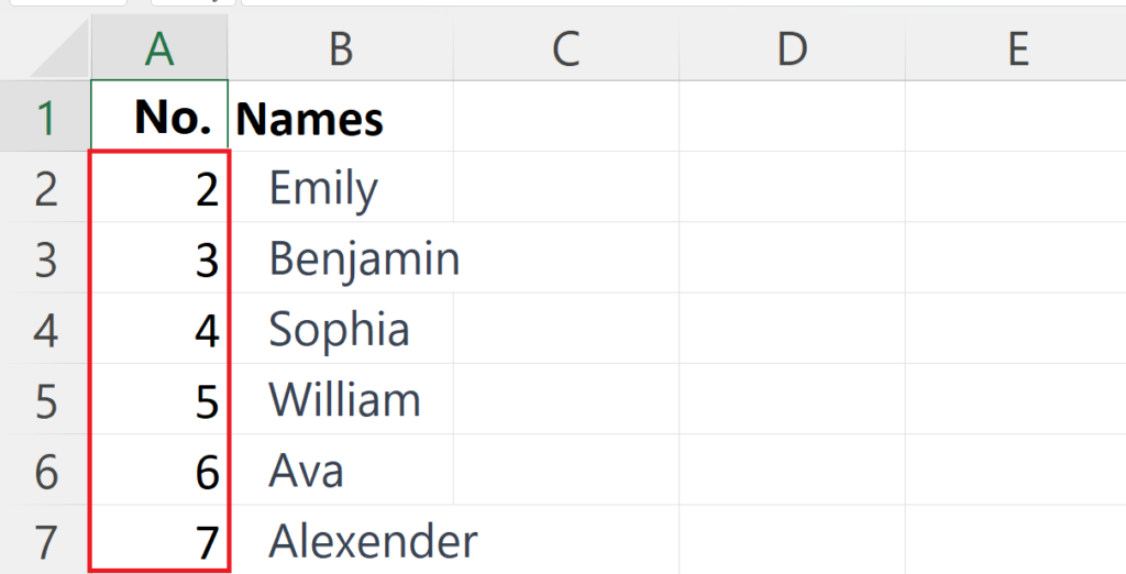
• Press the Enter key to generate the serial numbers.

Method 2: Add Serial Numbers Using the Text Box

Step 1 – Insert a Text Box

• Go to the Insert Tab in the menu bar.
• Click on the Text button and Select the Text Box option.
• The cursor will convert to an arrow.
• Click on the place where you want the Text Box to be.

Step 2 – Enter the Data

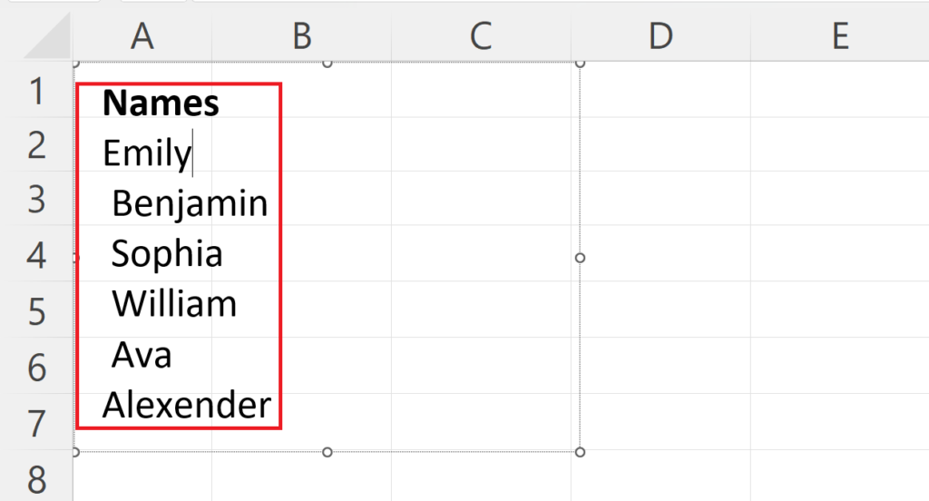
• Enter the data in the text box for which you want to add a numbered list.

Step 3 – Select the Data

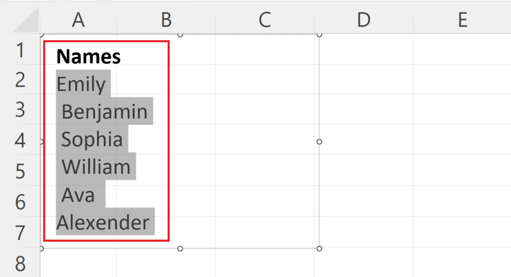
• Select the entered data.
• This can be done by shortcut keys i.e. CTRL + A

Step 4 – Right Click on the Data

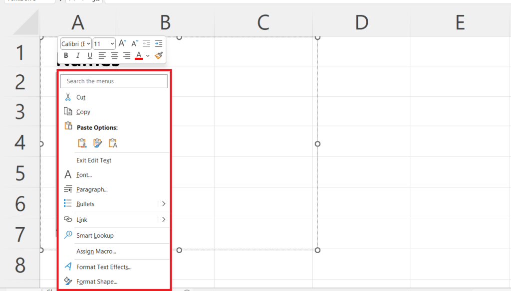
• Right-click on the selected data.
• A context menu will appear.

Step 5 – Click on the List Arrow with Bullets Option

• Click on the list arrow with the bullets option.
• Click on the Bullets and Numbering option.

Step 6 – Go to the Numbered Tab and Select the Numbered List

• Go to the numbered tab in the Bullets and Numbering dialog box.
• Select the Numbered List option.

Step 7 – Click on OK 

• Click on OK in the Bullets and Numbering dialog box.
• The numbered list will be created.

Method 3: Using the Autofill Feature to Generate Serial Numbers

Step 1 – Add the Number 1 in the First Cell 

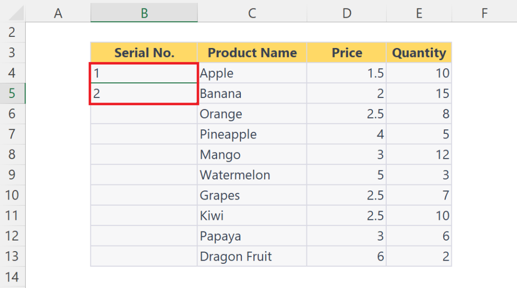
• Add the first two numbers manually in the first and second cells of the column in which you want to add serial numbers.

Step 2 – Select the Cells

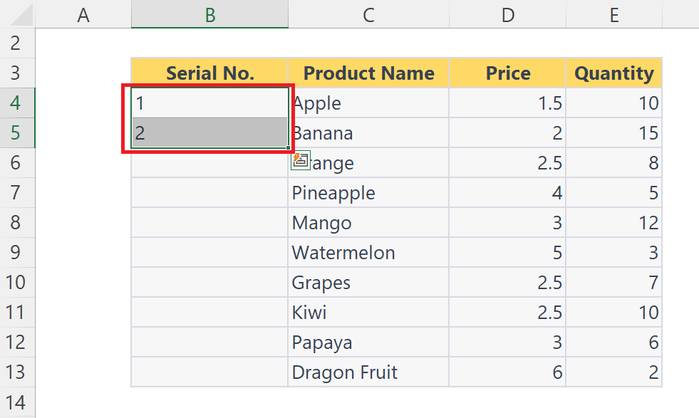
• Select the cells in which you have entered the numbers.

Step 3 – Hover the Cursor to the Right Bottom of the Cells

• Hover the cursor to the bottom right of the cells in which you have entered the number 1 and 2.
• The cursor will convert into a black plus sign.

Step 4 – Hold and Drag the Cursor Down and Drop 

• Hold and drag the cursor down over the cells till where you want to add the numbers.
• Drop the cursor.
• Numbers will be added automatically in the column.

Method 4: Add Serial Numbers Using SEQUENCE Function

We can also use the very handy and useful function called SEQUENCE to generate the serial numbers automatically in Excel.

The syntax of the SEQUENCE function is as follows; 

                                 SEQUENCE(rows, [columns], [start], [step])

Where;

rows:

This argument specifies the number of rows for which the serial numbers will be generated.

[columns]:

This argument is optional and it specifies the number of columns for which the serial numbers will be generated. By default, it is set to 1.

[start]:

This argument is optional and it specifies the number from where the sequence will start. By default, it is set to 1.

[step]:

This argument is optional and it specifies the step size by which the sequence will generate the next number. By default, it is set to 1.

Follow the steps mentioned below to learn how to use this function to generate the serial numbers in Excel.

Step 1 – Select a Blank Cell

• Select a blank cell in a column in which you want to add the serial numbers.

Step 2 – Place an Equals Sign

• Place an Equals sign in the blank cell.

Step 3 – Enter the SEQUENCE Function

• Enter the following formula using SEQUENCE function to generate serial numbers from 1 to 6.

=SEQUENCE(6) or =SEQUENCE(6,1,1,1)

Both formulas will work in the same way. In the first formula we didn’t enter the optional parameters and Excel will automatically assume them as 1. In the second formula we entered the optional parameters as well.

• This will generate the required serial numbers as shown above.