
How to add percentages in an Excel bar chart
 By
SpreadCheaters
By
SpreadCheaters
In this tutorial, we will learn how to add percentages in an Excel bar chart. Adding percentages to a bar chart in Microsoft Excel is an essential task that can be accomplished using the “Value from cells” option available in the Format Data labels pane.
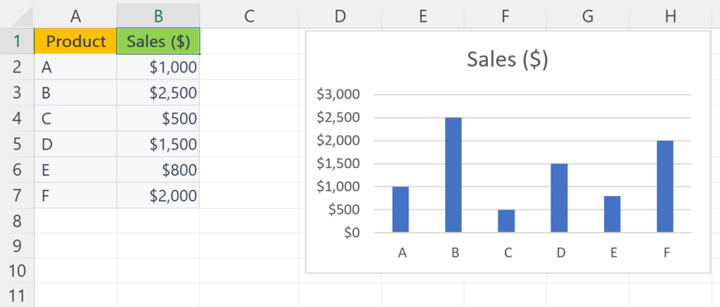
Currently, we have a bar chart of a data set showing sales of some products. We will be adding percentages of each sales figure in the bar chart.

Adding percentages to a bar chart in Excel can be a useful way to communicate the proportion of each category in the chart. This can help viewers to better understand the data and the relative importance of each category. By displaying the percentage values directly on the bars or using data labels, the chart becomes more informative and visually appealing.
Step 1 – Select a Blank Cell
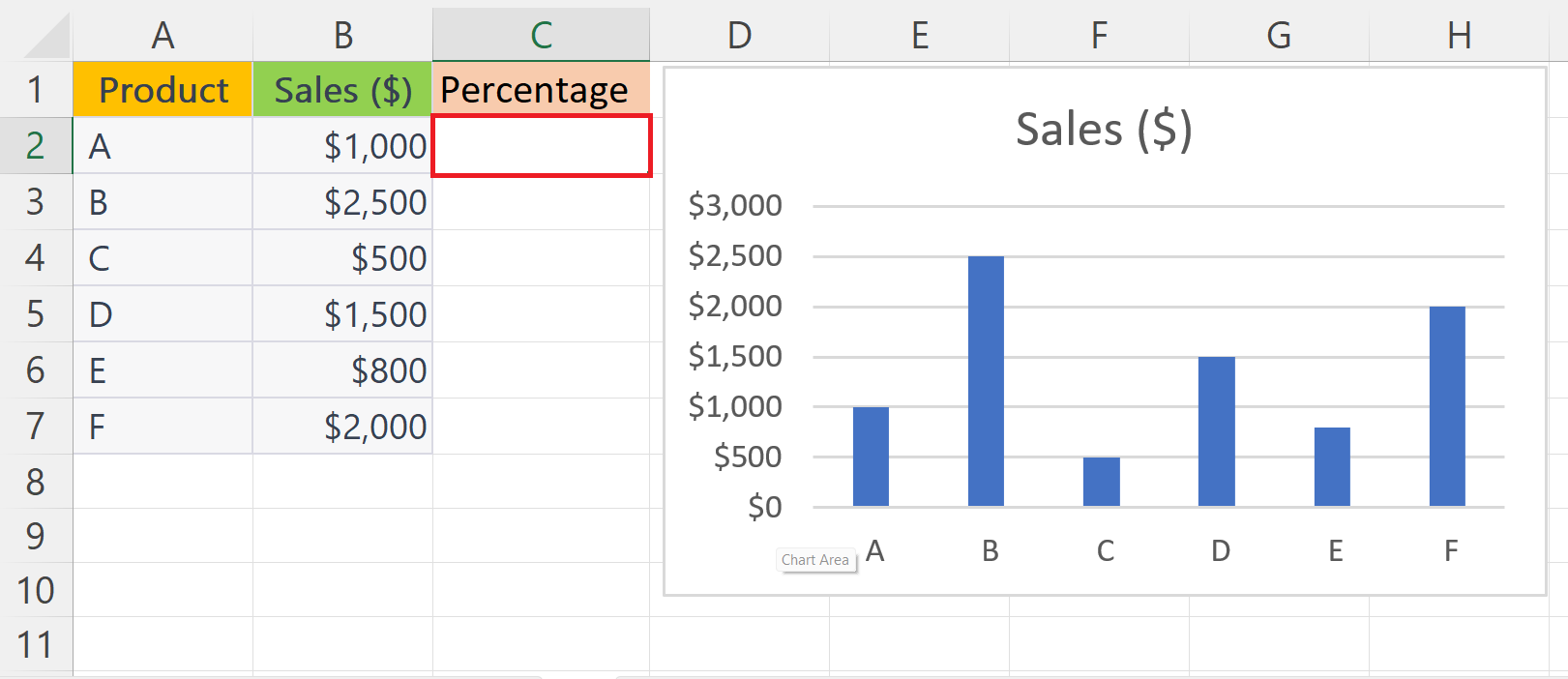
– Select a blank cell in the column next to the source data where to calculate the decimal value of each data point.
Step 2 – Convert the Value of the First Data Point to
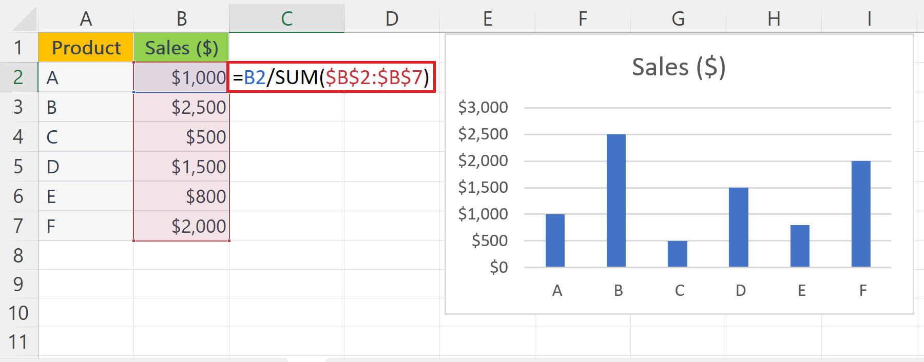
– Decimal in the Blank Cell
Place an Equals sign in the cell.
– Divide the value by the total of all values i.e. B2/SUM($B$2:$B$7)
– Where B2 is the cell containing the value of the data point and the SUM function calculates the total of the values of each data point.
Step 3 – Convert the Values of Each Data Point to Decimals
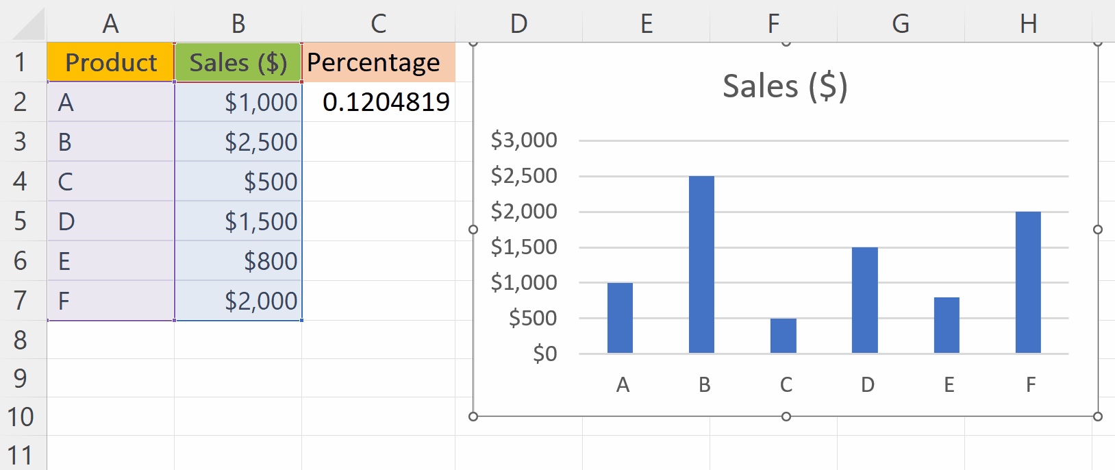
– Apply the formulae on the value of each data point using the autofill feature.
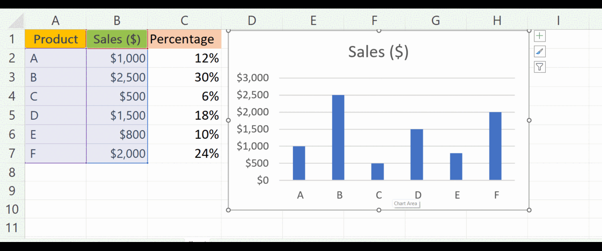
Step 4 – Convert the Decimal Values to Percentages
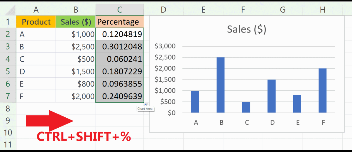
– Select all the cells containing the decimal values.
– Press CTRL + SHIFT + % keys.
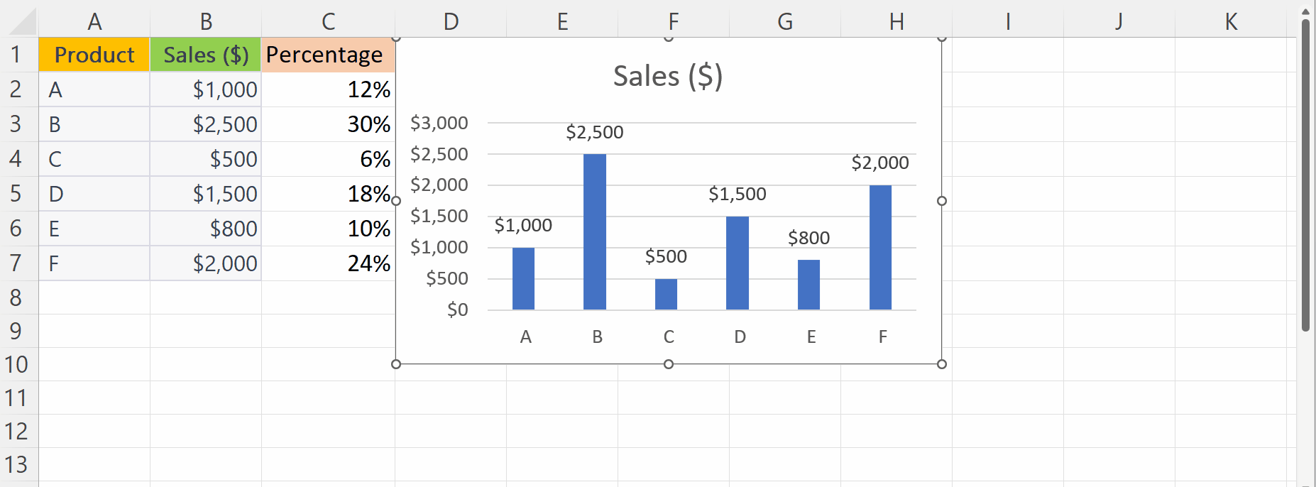
Step 5 – Enable Data Labels in the Bar Chart
– Click anywhere on the chart.
– A plus sign will appear on the right-top of the chart.
– Click on the plus sign and check the checkbox next to “Data Labels”.
– Data Labels will be added to the chart.
Step 6 – Double-Click on the Data Labels
– Double-click on any of the data labels in the chart.
– The Format Data Labels pane will open at the right of the window.
Step 7 – Go to the Label Option
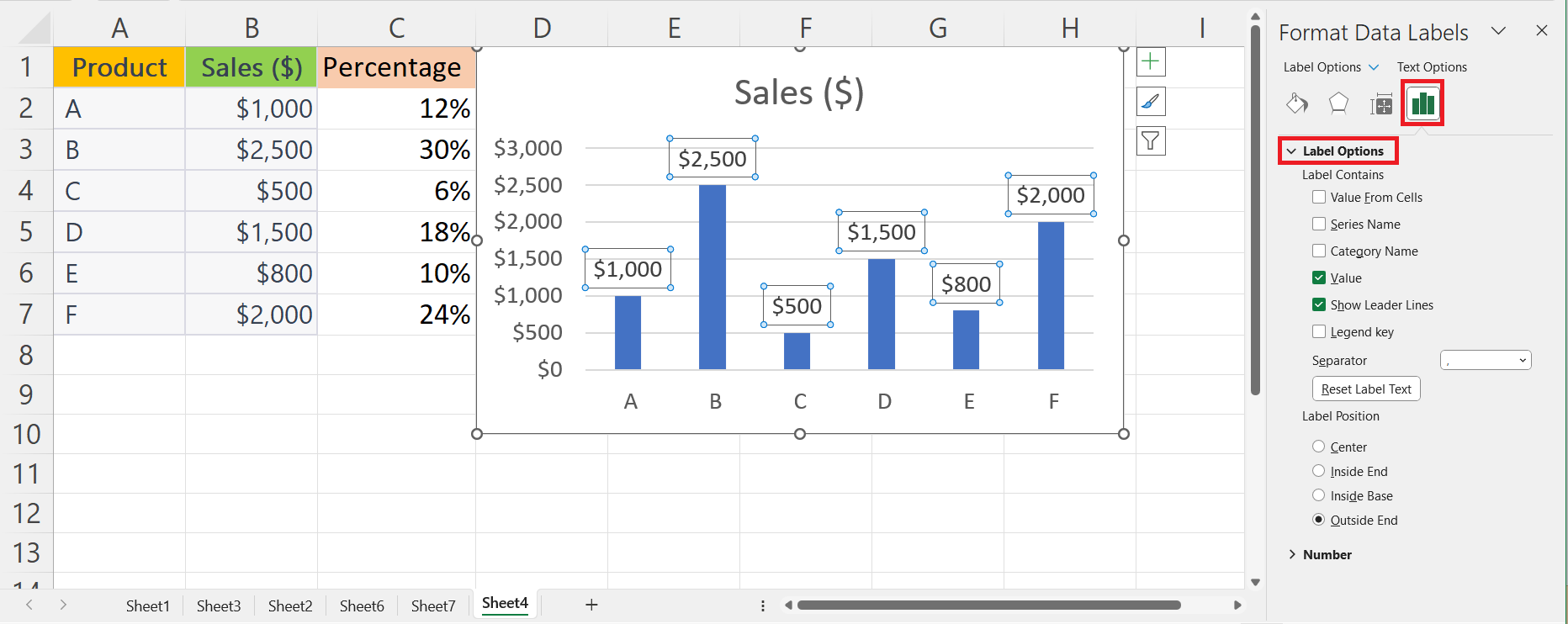
– Go to the Label Options by clicking on the Label Options icon.
Step 8 – Check the “Value from Cells Option”
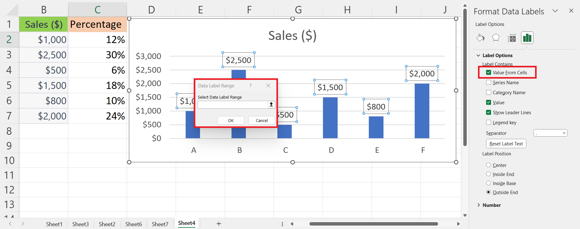
– Check the “Value from cells” option.
– The “Data Label Range” dialog box will appear.
Step 9 – Select the Range of Cells Containing the Decimal Values and Click on OK
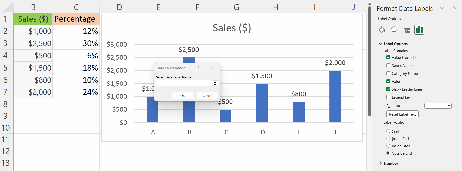
– Enter the range of cells containing the percentage values.
– Click on OK in the dialog box.


