
How to add months to a pivot table in Excel
 By
SpreadCheaters
By
SpreadCheaters
You can watch a video tutorial here.
Pivot tables are one of the most useful tools in Excel for summarizing and analyzing data. Pivot tables are built off a table or a dataset and can summarize rows or columns. When you have a pivot table that contains dates, you can group it according to months. This helps in organizing the table and in helping understand the table better.
Note: The dates in the source table must be formatted as dates so that Excel can extract the month.
Step 1 – Summon the menu
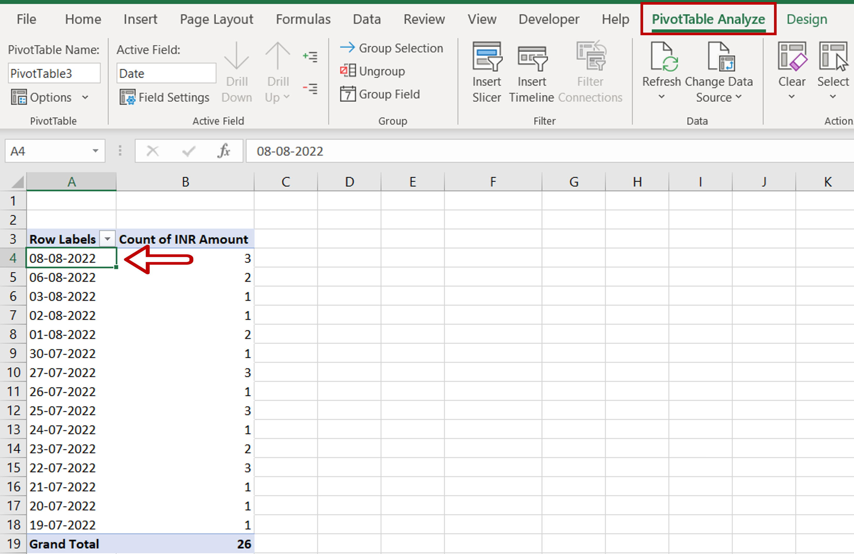
– Select any cell in the pivot table
– The PivotTable Analyze menu is displayed on the menu bar
Step 2 – Open the Grouping box
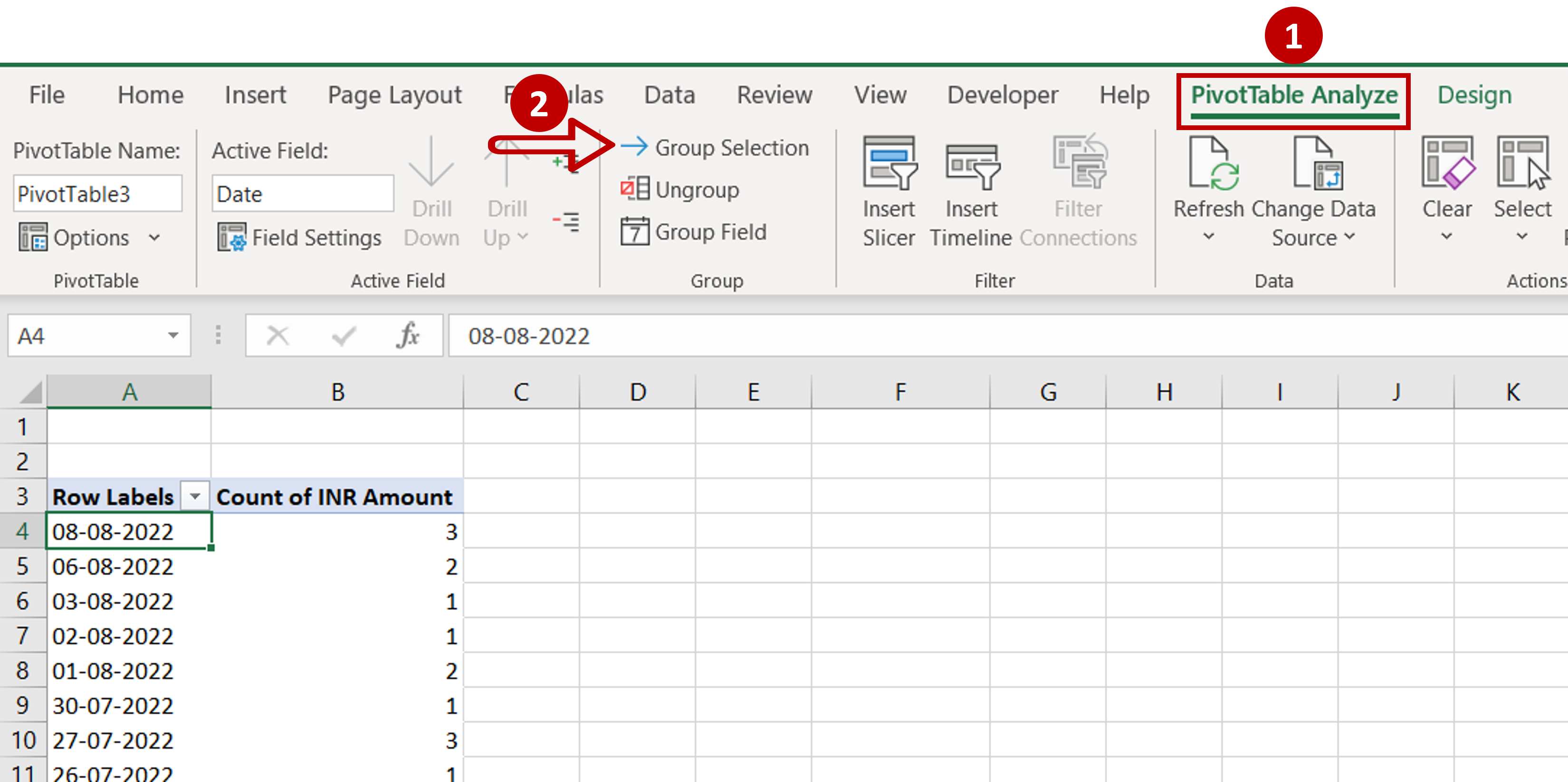
– Go to PivotTable Analyze > Group
– Click the Group Selection button
Step 3 – Choose the grouping option

– Choose Months and Days as the options to group by
– Click OK
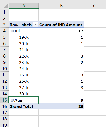
Step 4 – Check the result
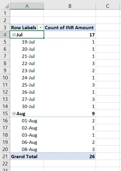
– The dates are grouped according to the months
– The months can be collapsed to hide the days


