How to add markers in Microsoft Excel

In Microsoft Excel, markers refer to small symbols or icons that appear on a chart to represent data points. These markers can take various forms, such as dots, squares, triangles, or other shapes, and can be customized to indicate different data series or categories.

In this tutorial, we will learn how to add markers in Microsoft Excel. To add markers in a chart in Excel, select the data points for which you want to add markers and then select the marker symbol from the “Chart Elements” or “Format” tabs. You can customize the appearance and size of the markers as well as their location relative to the data points.

Method 1: Adding Markers to Existing Chart

Step 1 – Right-Click on the Series

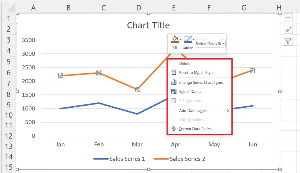
• Right-click on the Series in which you want to add the markers.
• A context menu will appear.

Step 2 – Click on the Format Data Series Option

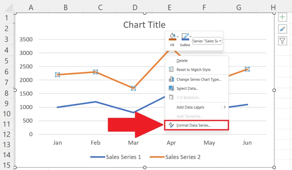
• Click on the Format Data Series option.
• Format Data Series Pane will open on the right of the window.

Step 3 – Click on the Fill & Line Button

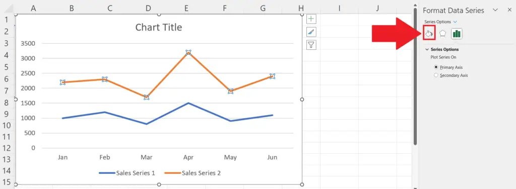
• Click on the Fill & Line button in the Series Options.

Step 4 – Choose the Marker Options

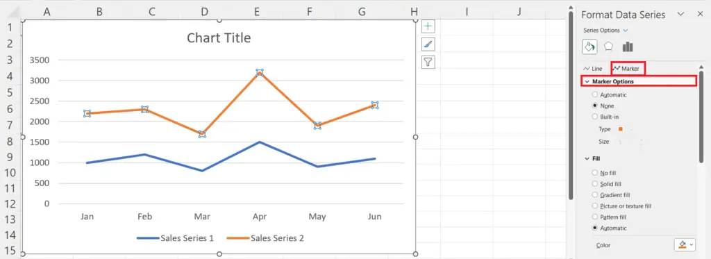
• Choose the Marker options.

Step 5 – Select the Built-in Option and Choose the Marker

• Select the Built-in option.
• The Type list arrow will be enabled.
• Select the type of marker in the Type list.

Step 6 – Close the Format Data Series Pane

• Close the Format Data Series pane.
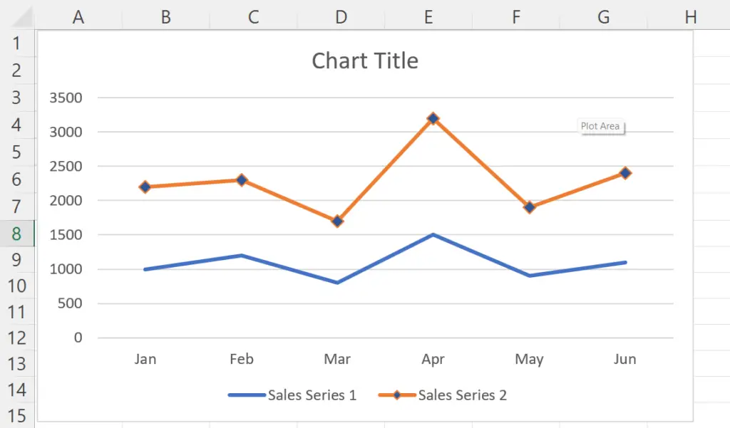
•  The chart would now include markers.

Method 2: Inserting a Chart with Pre-added Markers

Step 1 – Select the Data

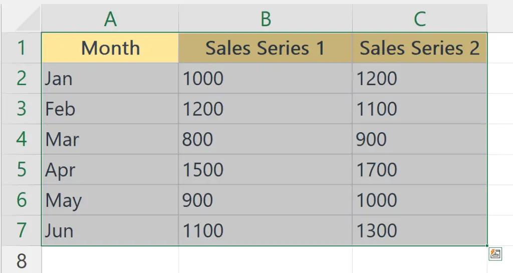
• Select the data range to insert a chart.

Step 2 – Go to the Insert Tab

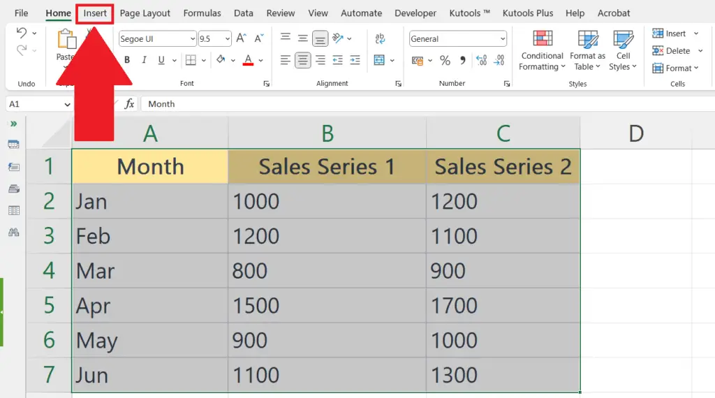
• Go to the Insert tab in the menu bar.

Step 3 – Click on a Chart with Markers

• Choose and click on a chart with pre-added markers.