
How to add a title to a Pivot Chart in Microsoft Excel
 By
SpreadCheaters
By
SpreadCheaters
Pivot charts are an essential tool in data analysis as they allow users to visualize complex data sets in a clear and concise manner. A pivot chart provides the ability to communicate complex data in a way that is easily understandable. This is where the title of a pivot chart becomes crucial. A clear and concise title can provide context to the data being presented and help users quickly understand the chart’s purpose.
In this tutorial, we will learn how to add a title to a pivot chart in Microsoft Excel. There are a few ways to add a title to a pivot chart in Excel. One way is to add a title to a pivot chart using the “Add Chart Elements” option in the “Design” tab. Another method is to use the “Chart Elements” green plus sign on the top right of the pivot chart.
Method 1: Adding a title using the Design Tab
Step 1 – Click on anywhere on the Pivot Chart
Click anywhere on the pivot chart to activate the Design tab in the menu bar.
Step 2 – Go to the Design Tab
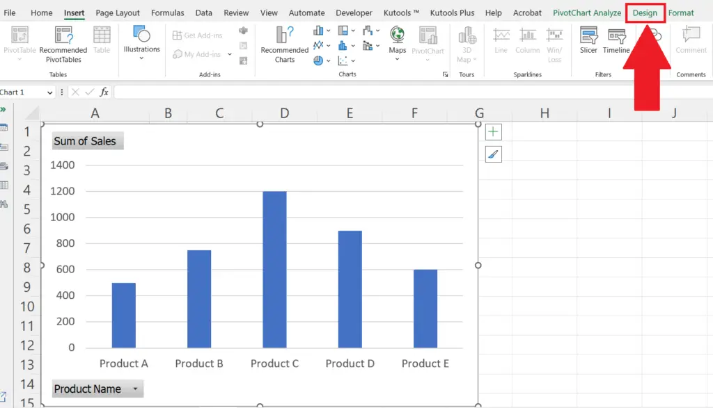
Go to the Design tab in the menu bar.
Step 3 – Click on the “Add Chart Elements” Button
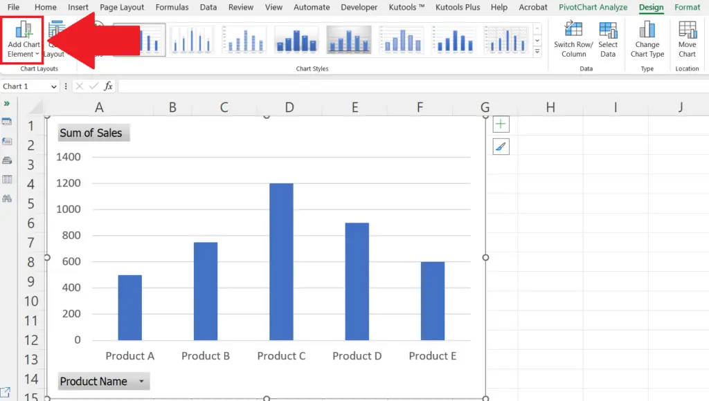
Click on the “Add Chart Elements” button on the left of the ribbon.
A drop-down list will appear.
Step 4 – Click on the “Add Title” Option
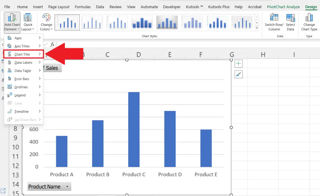
Click on the “Add Title” option in the drop-down list.
Step 5 – Select Where the Title Is to be Added in the Pivot Chart
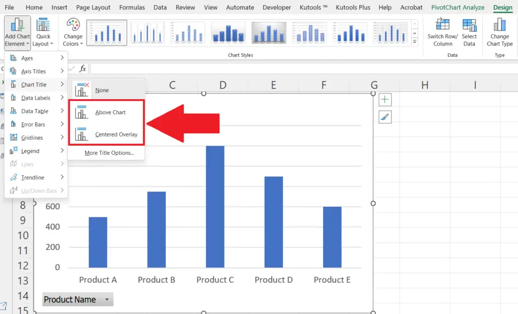
Select the required option according to where the title is to be added in the Pivot Chart i.e. Above the Chart.
The title will be added to the pivot chart.
Step 6 – Right-Click on the Title and Click on the Edit Text Option

Right-click on the added title and a context menu will appear.
Click on the Edit Text option.
Add suitable text to the title.
Method 2: Using the “Chart Elements” Plus Sign
Step 1 – Click Anywhere on the Chart
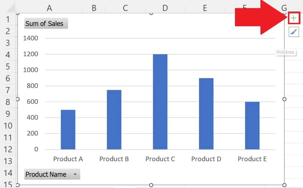
Click on anywhere on the chart.
A green plus sign will appear on the top right corner of the Pivot Chart.
Step 2 – Click on the “Chart Elements” Plus Sign

Click on the green plus sign in the top right corner of the pivot chart.
A chart elements list will appear.
Step 3 – Check the Box Prior to the “Chart Title” Option
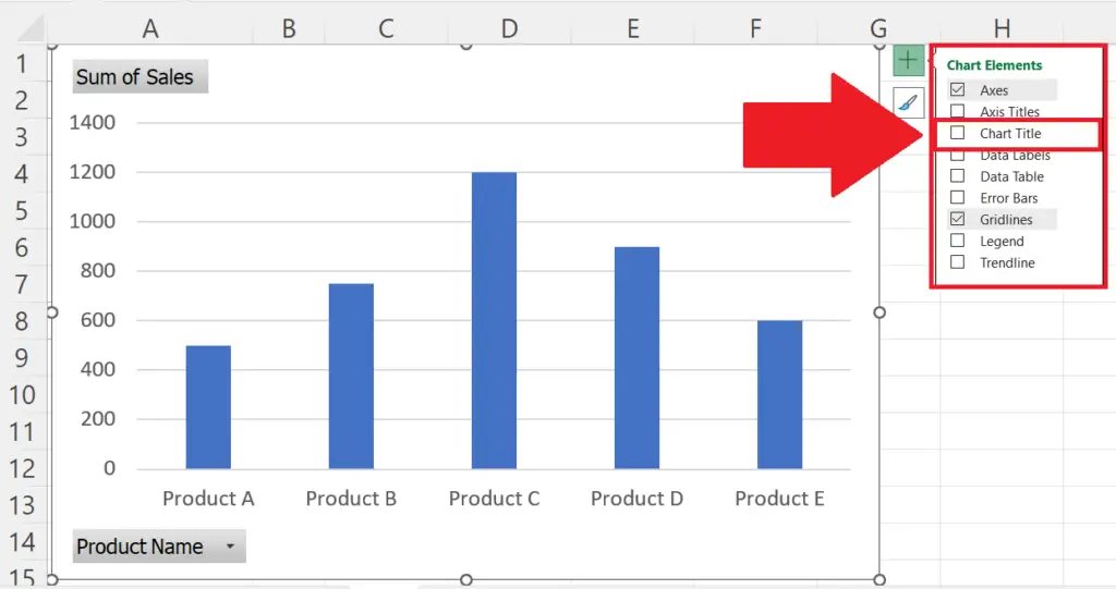
Check the box prior to the “Chart Title” option in the list,
The title will be added to the pivot chart.
You may select the location of the title in the pivot chart by clicking on the list arrow next to the “Chart Tile” option.
Step 4 – Right-Click on the Title and Click on the Edit Text Option
Right-click on the added title and a context menu will appear.
Click on the Edit Text option.
Add suitable text to the title.


