How to add a specific text to all cells in Excel + remove them

Have you ever had a list with a hundred items and you’ll need to add a specific text to each and every one of them? It sounds troubling if you do it one by one. But worry not, this tutorial got you covered. We will learn how to add a specific text to the range of cells. And added bonus, we will also learn to remove a specific text in all the selected cells. 

Add a specific text to all the selected cells

Excel gave us so many options to do this. We will learn the top three most easiest way to achieve this:

• Flash Fill
• CONCATENATE function
• TEXTJOIN function

Flash Fill

Flash Fill is one of the most helpful features in Excel. It can fill your list in a flash when it senses a pattern. We can use this advantage to add a specific text to the cells. Just follow these easy steps:

Step 1 – Draw the pattern

• To draw the pattern, we need to fill the first cell ourselves. Enter the name with the salutation.

Ms. Katherine Griffin

Step 2 – Use the Flash Fill

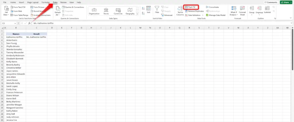
• Go to DATA
• Along the Data Tools, click on the Flash Fill.

Alternative Step 2 – Use the Flash Fill

• Press CTRL+E on your keyboard.

CONCATENATE Function

The word “concatenate” means to link things together in a chain or series. The function CONCATENATE means the same. We are using the function to link together the arguments we entered. Here’s how we’re going to use this to add a specific text to all the cells.

Step 1 – Insert Function

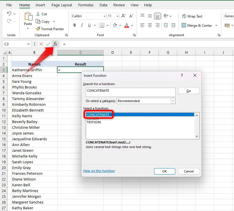
• Open the Insert Function dialogue box by clicking the fx symbol at the left side of the formula bar
• Search for “CONCATENATE” in the search bar
• Double click on the function 

Step 2 – Enter the arguments

• We want to put the salutation before the name, therefore, input “Ms. “ as Text1. Remember to put a space before closing the quotation marks so there will be a space between the salutation and the name.
• Text2 will be the name, so  select the name on Column B
• Click OK

Step 2 – Apply the formula to all the cells

• Extend the formula down to the bottom of our list by double-clicking the small square in the cell with formula.

TEXTJOIN Function

The TEXTJOIN function comes from the words “text” and “join”. Using this means we are joining together the text we selected. It has the same function as concatenate but with more specific arguments. The syntax of this function is: TEXTJOIN(delimiter,ignore_empty,text1,[text2],…). The argument delimiter is what we set as a separator between the texts we are joining. It is entered into Excel enclosed by double quotes. Then, the ignore_empty argument is answering the question if we should ignore the empty cells. The value of this argument should only be TRUE or FALSE. The next arguments are the text that we wish to join together. We can join a maximum of 252 strings in a cell. Now let’s dive into the formula.

Step 1 – Insert Function

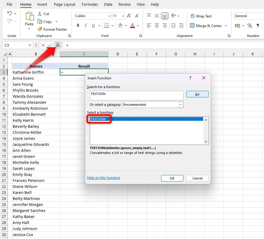
• Open the Insert Function dialogue box by clicking the fx symbol at the left side of the formula bar
• Search for “TEXTJOIN” in the search bar
• Double click on the function 

Step 2 – Set the condition arguments

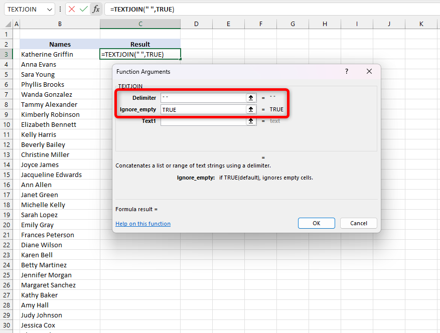
• We want a space between the salutation and the name, so we are going to set our delimiter a space inside the double quotes. Like this:

“ “

• We will ignore the empty cells so input “TRUE” on the ignore_text function

Step 3 – Set the text arguments

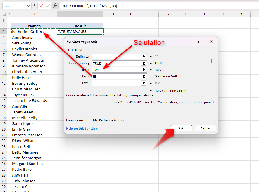
• The first part of the text result is the salutation so enter “Ms.” as our Text1
• Our Text2 will be the name so select the cell from the Column B.
• These two text strings are the only component we want. Therefore we are done and we can click OK.

Step 4 – Extend the formula

• Extend the formula until the list ends.

Remove a specific text in all the selected cells

For this task, we will use an Excel feature called ‘Find and Replace’. As the terms suggest, it is used to find and replace. In our example we have a list of names with salutation and we want to remove it using the ‘Replace’ feature.

Step 1 – Select the cells that contain the specific text

• In the example, all the names in the list have a salutation. So we are going to press CTRL+SHIFT+Down Arrow on your keyboard to select all the cells in the list

Step 2 – Open the ‘Find and Replace’ dialogue box

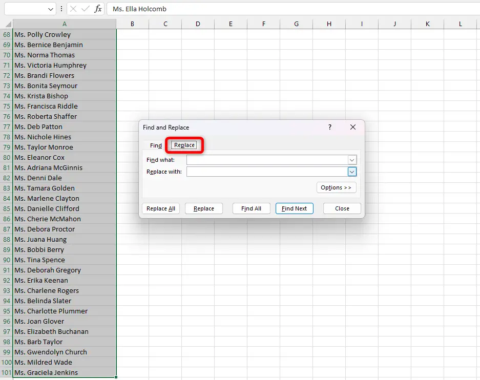
• Open the ‘Find and Replace’ dialogue box by pressing CTRL+H on your keyboard
• It will directly go to the “Replace” tab

Step 3 – Type the text you want to remove

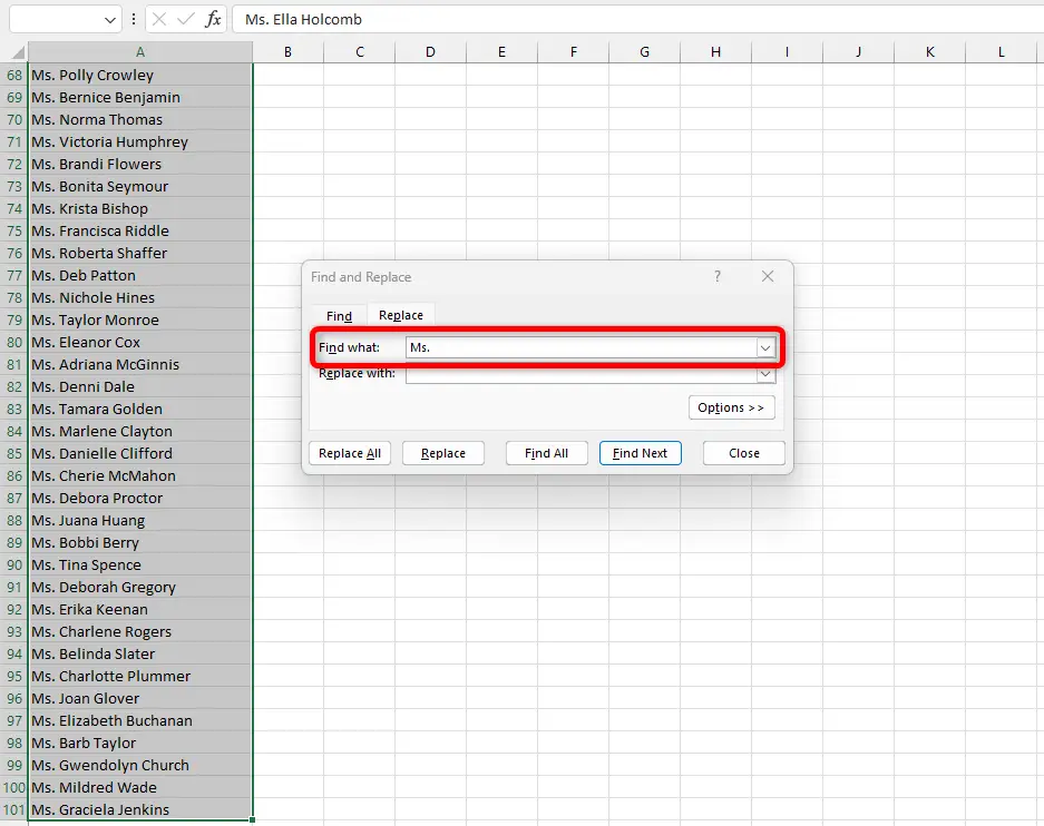
• In our example, we want to remove the salutation so we will type ‘Ms. ‘ in the ‘Find what:’ bar
• Remember to put a space at the end, because we want only the names to retain in the cells

Step 4 – Replace All

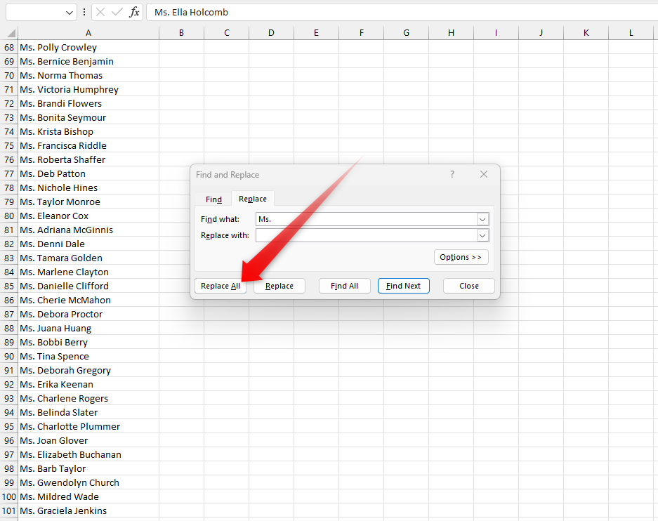
• We will leave the ‘Replace with:’ bar empty because we want the salutations to be replaced with nothing.
• Click on the ‘Replace All’ in the lower left of the dialogue box.

Step 5 – Confirmation Prompt

• Upon clicking ‘Replace All’, a confirmation prompt will appear telling that the replacement has been completed.
• Click OK on the prompt
• Close the ‘Find and Replace’ dialogue box