How to add a comma in Microsoft Excel between names

Adding a comma between names in Microsoft Excel is a way to separate the first name and last name of an individual in a single cell. This is useful when you have a list of names in a spreadsheet and you want to separate them into two separate columns. This can be useful for organizing and analyzing data.

In this tutorial, we will learn how to add a comma in Microsoft Excel between names. Excel provides multiple approaches to adding a comma between names. One of the most commonly used methods is to employ the Find & Replace feature. Additionally, functions like SUBSTITUTE or FIND and REPLACE can also be used for this purpose. Another quick and easy way to add commas between names in Excel is by leveraging the Flash Fill feature.

We have a data set representing 5 names. We want to add a comma between each name.

Method 1: Using the Flash Fill Feature

Step 1 – Enter a Comma in the First Name

• Enter a comma “ , ” in the first name manually.

Step 2 –  Select the Adjacent Cell

• Select the adjacent cell where the next name after adding the comma is to be placed.

Step 3 – Press the CTRL + E Keys

• Press the CTRL + E shortcut keys to use the Flash Fill.
• This will add a comma to each of the listed names.

Method 2: Using the SUBSTITUTE Function

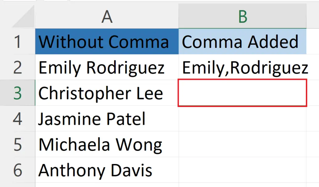
Step 1 – Select a Blank Cell and Place an Equals Sign

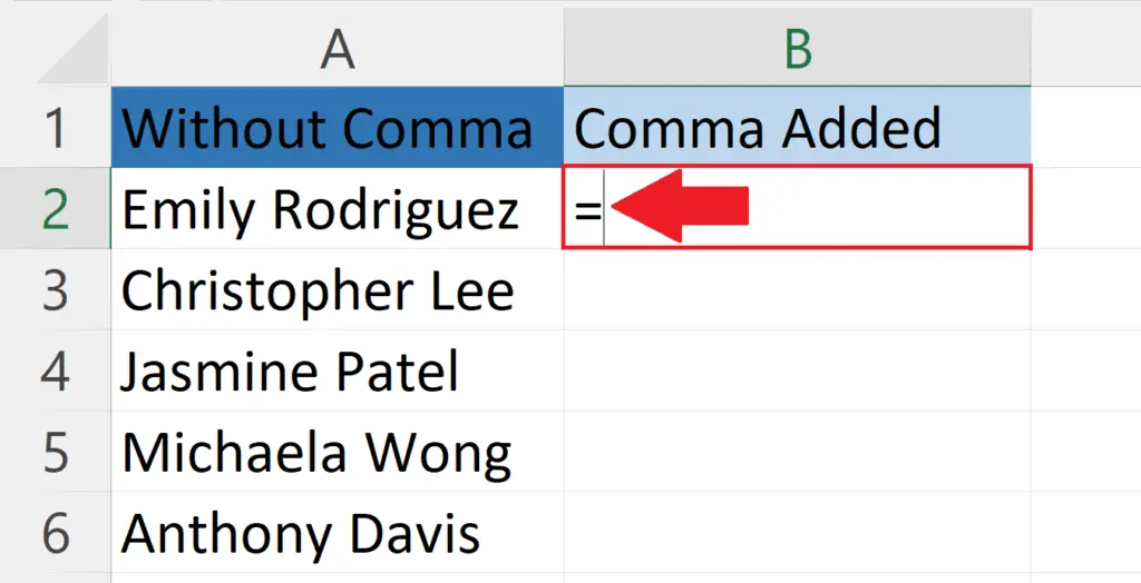
• Select a blank cell where you want to place the name after adding a comma.
• Place an Equals sign in the blank cell.

Step 2 – Enter the SUBSTITUTE Function

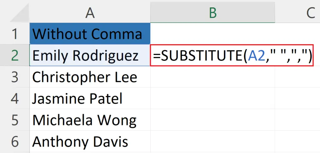
• Enter the SUBSTITUTE function next to the equals sign.
• The syntax of the SUBSTITUTE function will be: 

                     SUBSTITUTE( A2, “ ”, “,” )

The first argument i.e. A2 is the cell containing the name.

The second argument i.e.  “ ”, is the text to be replaced.

The third argument i.e. “,” is the the new text to be added.

Step 3 – Press the Enter Key

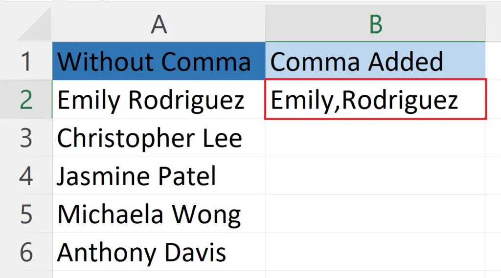
• Press the Enter key to add the comma in the name.

Step 4 – Use the Autofill to Apply the Function on Each Name

• Use the Autofill feature to apply the function on each name listed.

Method 3: Using the Find & Replace Feature

Step 1 – Select the Range of Cells

• Copy paset the original data to another column if you want to keep the original data intact. Otherwise, select the range of cells containing the names.

Step 2 – Click on the Find & Select Button

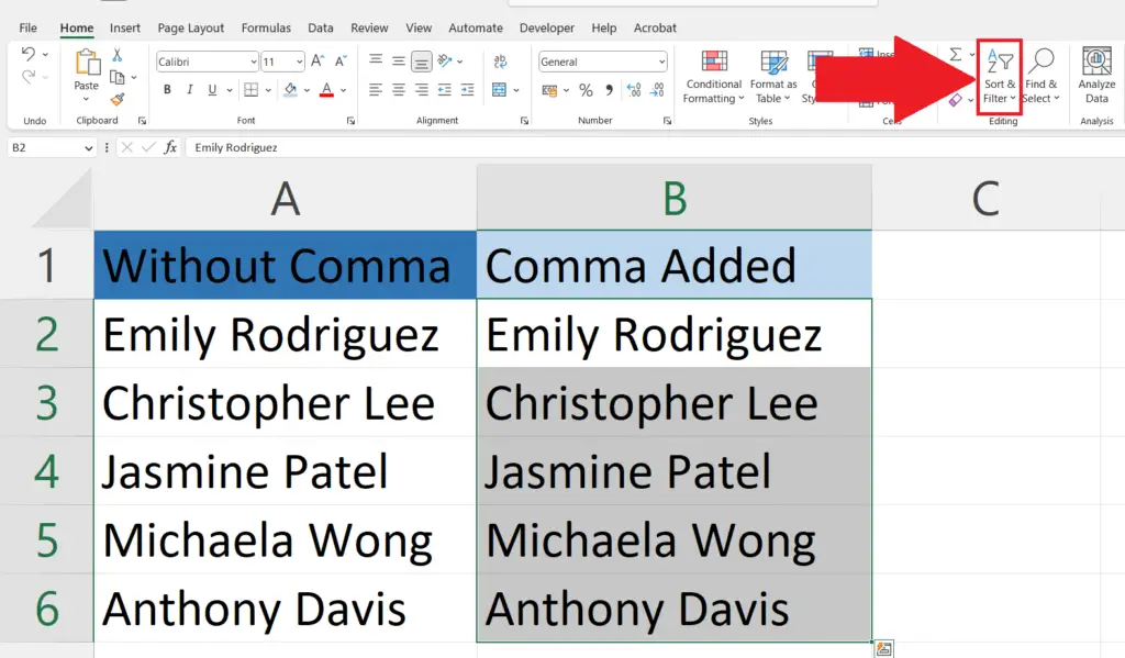
• Click on the “Find & Select” button in the “Editing” section of the Home tab.
• A drop-down menu will appear.

Step 3 – Click on Replace Option

• Click on the Replace option in the drop-down menu.
• The Find & Replace dialog box will open.
• This can also be done by simply pressing the “CTRL + H” shortcut keys.

Step 4 – Enter a Space 

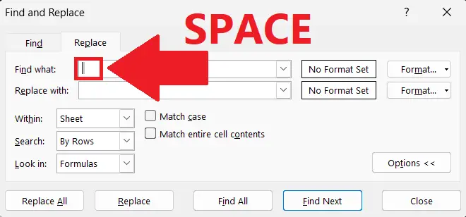
• Enter a Space in the “Find what:” field.

Step 5 – Enter a Comma 

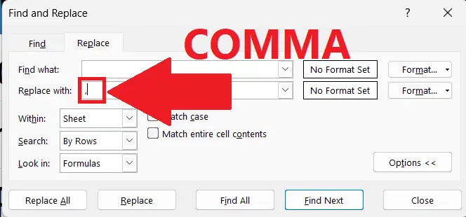
• Enter a comma in the “Replace with:” field.

Step 6 – Click on Replace All Option

• Click on the Replace All option in the Find & Replace dialog box.
• A comma will be added between each name in the selected range.