How to add 60 days to a date in Excel 

Adding days to a certain date in Excel can be a useful way to perform various calculations related to time and dates. If you are planning an event that will take place in the future, you can use Excel to calculate the date and time by adding the number of days to the start date.

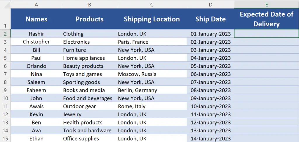
The example given below has a dataset containing information about sales of different products and their date of shipping. Now, we want to calculate the expected date of delivery which is 60 days as per the company’s policy. We will learn how to add some days to a certain date in Excel by using simple methods.

Method 1 – Add days to the dates directly as numbers

In Excel, dates are processed as serial numbers, allowing us to directly add numerical values to days. However, to add years and months, a specific formula must be used, which we will cover later in this tutorial.

Step 1 – Add days like a number to the date

• We will input a basic formula into the “Expected Dates of Delivery” column of our dataset which is actually column E.
• Firstly, press the = button on your keyboard.
• Then, select the cell in which the starting date is mentioned e.g., it is D2 in this case.
• After that, write +60 which will add 60 days to the date in D2.
• Now, your formula would look like this, D2+90.
• Then, press Enter button on your keyboard and 60 days will be added to the date.

Step 2 – Implement the formula to the whole data range

• For implementing the same formula to the whole column, move your cursor over the cell in which 60 days are added to date e.g., it is E2 in this case.
• Then, move your cursor to the bottom right corner of the cell until your cursor changes shape to + which is actually called the fill handle.
• Now, double-click on the fill handle and the same formula will be applied to the complete range as shown below.

Method 2 – Add days to the dates using the DATE function

The DATE function in Excel allows you to add days to your dates using a simple syntax which is as follows:

DATE(year, month, day)

Where;

year: 

Year is a numeric value that is written either in the form of a four-digit value or a two-digit value. For example, 2023 will be a four-digit value representing the year and if you write 23, Excel will interpret it as 2023 according to the current century which is the 21^st century.

month: 

This parameter is a numeric value representing the month starting from 1 which means January to 12 which means December.

day: 

The last parameter is a numeric value that represents the day of the month, from 1 to 31.

Step 1 – Create a formula using the DATE function

• Select the cell in which you want to write the date in which 60 days are added.
• Then, press the = button on your keyboard.
• After that write this formula,

=DATE(YEAR(D2), MONTH(D2), DAY(D2)+60)

This will add 60 days to the DAY parameter.

• Now, press Enter and you’ll get the desired result.

Step 2 – Implement the formula to the whole data range

• For implementing the same formula to the whole column, move your cursor over the cell in which 60 days are added to date e.g., it is E2 in this case.
• Then, move your cursor to the bottom right corner of the cell until your cursor changes shape to + which is actually called the fill handle.
• Now, double-click on the fill handle and the same formula will be applied to the complete range as shown below.