How to add 15 minutes to a time in Excel 

When working in Excel, we often need to add or subtract time. Excel can do many things over time, such as addition and subtraction over time. Excel can be used to track time spent on a task or project. Excel makes it easy to track all working hours by calculating the total time spent on the task by entering the start and end times. Excel can perform time-based calculations, such as calculating the average time between tasks, the difference between two tasks, or the time it takes to complete a project. Excel can create schedules or calendars that often involve working with chronological data. 

There are many ways to add minutes to a time in Excel. Among all that, this tutorial describes two simple and easy ways to add time. One way is adding minutes directly to the time. Another way is to use the TIME function for increasing the time by any amount of minutes. 

Method 1 – Adding 15 minutes to a time using the formula 

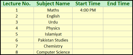
To understand the formula used, we must first understand its logic. In Excel, time values are represented as decimal values where one day is equal to the value of 1.0. In this representation, the fractional part of the value represents the time. For example, 0.5 represents 12:00 PM, which is half of a day. Therefore, if we add 15 directly to a time value it will add 15 days to it.  

So, as a day has 24 hours and an hour is 60 minutes, then a day will be (24*60) = 1440 minutes. Therefore, we’ll have to use = (time) + (15/1440) for adding 15 minutes. Let’s consider the following dataset that contains a timetable of an academy, where each lecture is 15 minutes long. So we need to add 15 minutes to the start time to calculate the end time of each lecture: 

Step 1 – Format the column for “Start Time” and “End Time” as Time 

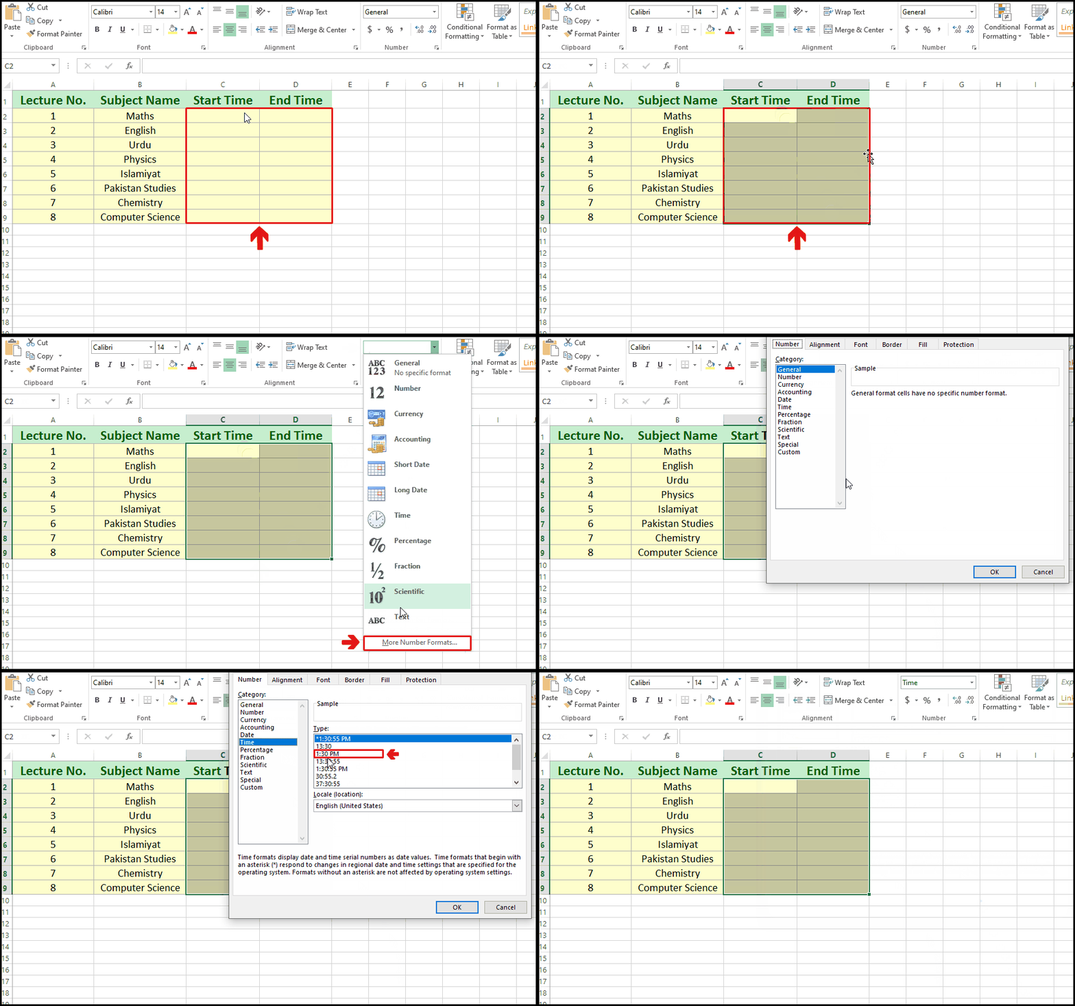
• Select the columns for “Start Time” and “End Time”. 
• Click on the down arrow in the “Number” group from the “Home” tab. 
• Click on “More Number formats…”. 
• From categories, choose Time. 

• Click on 1:30 PM. 
• Click on OK. 

Step 2 – Use the formula to add minutes directly to a time 

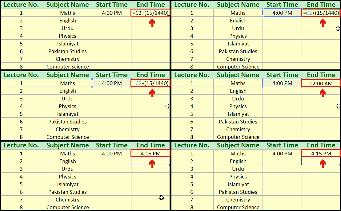
• As described above, we need to add (minutes/1440) to the time value in order to add minutes to it. 
• In this case, the used formula is =C2+(15/1440). 
• Write the formula in the cell where you want the result of the sum. 
• Press enter key. 
• 15 minutes will be added to the time. 

Step 3 – Write the End Time of Lecture No. 1 as the Start Time of Lecture No. 2 

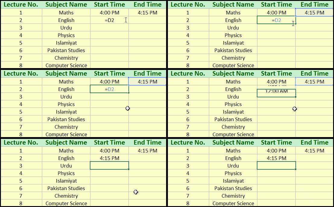
• To write the Ending Time of the first lecture in place of the Starting Time of the second lecture, we need to write =(end time) in the Start Time column. 
• In this case, the formula is  =D2. 

• Write =D2 in the start time of the second lecture. 

Step 4 – Use the Fill handle to calculate Start and End times for all lectures 

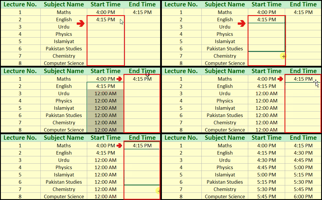
• Move your cursor to the bottom right of the cell where the formula is already applied. 
• Drag the Fill handle up to lecture no.8 to calculate the Staring times of all lectures. 
• Follow the same steps for the End Time column. 

Method 2 – Adding 15 minutes using the TIME Function 

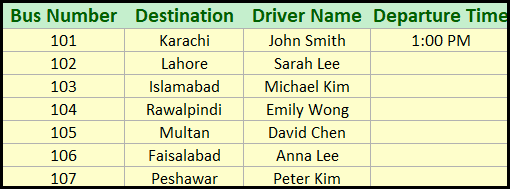
Another method to add hours, minutes, and seconds to a time is to use the TIME function. TIME function has the syntax =TIME(hours, minutes, seconds). This indicates that the parameters of this function are three: hours, minutes, and seconds. In the “hours” place, we need to write the number of hours to be added. The same goes for minutes and seconds. Consider the following dataset that contains the departure schedule of a bus station, where a bus departs every 15 minutes: 

Step 1 – Format the “Departure Time” column as Time 

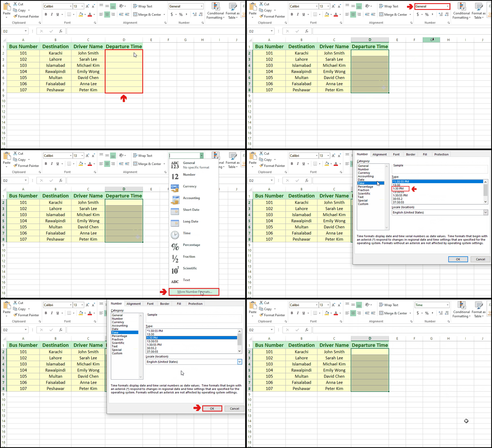
• Select the “Departure Time”  column. 
• Click on the down arrow in the “Number” group in the “Home” tab. 
• Click on “More Number Formats…”. 
• From the categories, click on Time. 

• Choose 1:30 PM. 
• Click OK. 

Step 2 – Use the TIME function for adding 15 minutes 

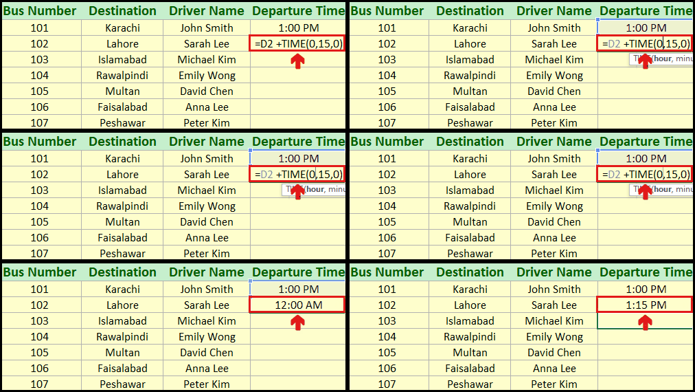
• Create an appropriate formula for adding 15 minutes to a time value using the TIME function. 
• In this case, the used formula is =D2+TIME(00,15,00). 
• Write the formula in the cell where you want the result. 

• Press Enter key. 

Step 3 – Use the Fill handle to calculate departure times for all buses 

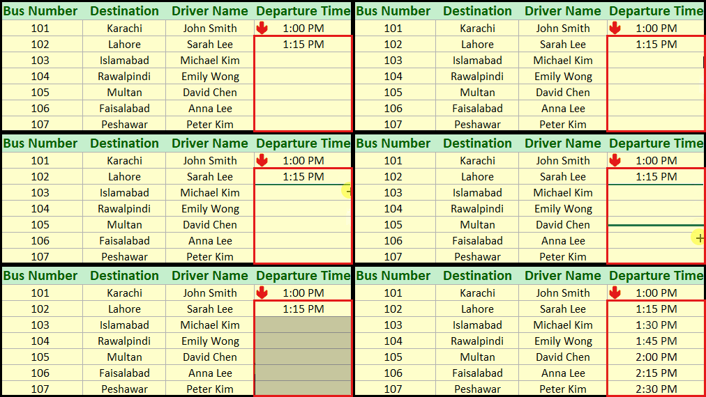
• Move your cursor to the bottom right of the cell where the formula had already been applied. 
• Drag the Fill handle up to the last bus to find out departure times for all buses.