
How to accounting format in Excel
 By
SpreadCheaters
By
SpreadCheaters
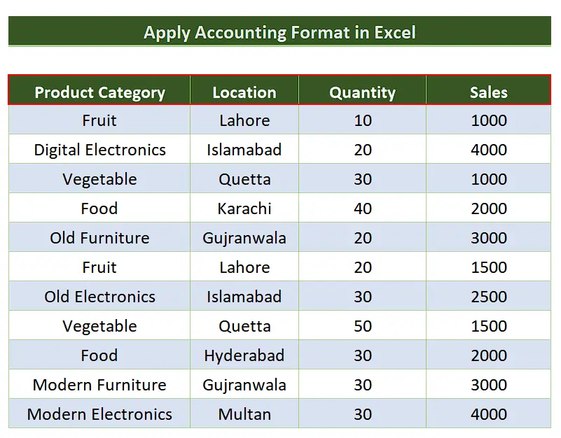
In today’s tutorial we are going to learn how to apply Accounting Format to numbers in Excel. Let’s take a look at the following sales dataset.
We have the sales data in the last column to which we’ll apply the accounting format. There are various methods which can do the same thing i.e., apply accounting format to the numbers. Let’s explore these one by one.

Microsoft Excel is one of the best tools which provides so many features to handle and manipulate versatile data with its efficient tools and functions. It also provides many built-in tools and features that can help the data analysts in visualizing data in the best possible ways. One such feature is the ability of Excel to apply various data formats on datasets to categorize the data properly.
Step 1 – Apply the accounting format using shortcut key CTRL+1
– Select the whole sales columns leaving behind the header of your dataset.
– Use the shortcut key CTRL+1 to open the Format Cells dialog box.
– Choose the Accounting format from the Category options.
– Now you can choose the number of decimal places to be used and symbols for the currency depending upon your locale as shown below.
– Then press the OK button and it will apply the accounting format to the whole column.
Step 2 – Apply the accounting format using context menu
– Select the whole sales columns leaving behind the header of your dataset.
– Right click and choose the Format Cells option from the context menu.
– This will open up the Format Cells dialog box.
– Choose the Accounting format from the Category options.
– Now you can choose the number of decimal places to be used and symbols for the currency depending upon your locale as shown below.
– Then press the OK button and it will apply the accounting format to the whole column.
Step 3 – Apply the accounting format from Main Menu
– Select the whole sales columns leaving behind the header of your dataset.
– Now on the Home tab go to the Cells group and click on the Format dropdown.
– Choose Format Cells from the available options.
– This will open up the Format Cells dialog box.
– Choose the Accounting format from the Category options.
– Now you can choose the number of decimal places to be used and symbols for the currency depending upon your locale as shown below.
– Then press the OK button and it will apply the accounting format to the whole column.


