
How does XLOOKUP function work in Microsoft Excel
 By
SpreadCheaters
By
SpreadCheaters

In this tutorial we will learn how XLOOKUP function works in Microsoft Excel. The XLOOKUP function in Excel is used to find a particular value in a table or array and then return a corresponding value from another column in the same table or array. Let’s understand the syntax of XLOOKUP function first.
Syntax of XLOOKUP
The basic syntax of the XLOOKUP function is as follows:
=XLOOKUP(lookup_value, lookup_array, return_array, [if_not_found], [match_mode], [search_mode])
The XLOOKUP function requires at least three arguments: lookup_value, lookup_array, and return_array. The match_mode and search_mode arguments are optional.
Lookup Value: The first argument, lookup_value, is the value that you want to search for. This value can be a number, text, or a cell reference.
Lookup Array: The second argument, lookup_array, is the range or array of cells that you want to search in. The lookup_array must have at least two columns: one column for the lookup values, and another column for the return values.
Return Array: The third argument, return_array, is the range or array of cells that contains the values that you want to return. The return_array can have one or more columns.
[if_not_found]: You can add an optional argument to the XLOOKUP function to specify what should happen if the lookup_value is not found in the lookup_array. This argument is called [if_not_found] and can be added as the last argument in the function.
Match Mode: The fourth argument, match_mode, is optional and specifies the type of match you want to use. There are four options:
- 0 or omitted: Exact match (default)
- 1: Exact or next smallest match
- -1: Exact or next largest match
- 2: Wildcard match
Search Mode: The fifth argument, search_mode, is optional and specifies whether to search for the lookup_value from the beginning or end of the lookup_array. There are two options:
1 or omitted: Search from the beginning (default)
-1: Search from the end
The XLOOKUP function returns the value that corresponds to the lookup_value in the return_array. If the lookup_value is not found in the lookup_array, the function can return an optional default value or an error message.
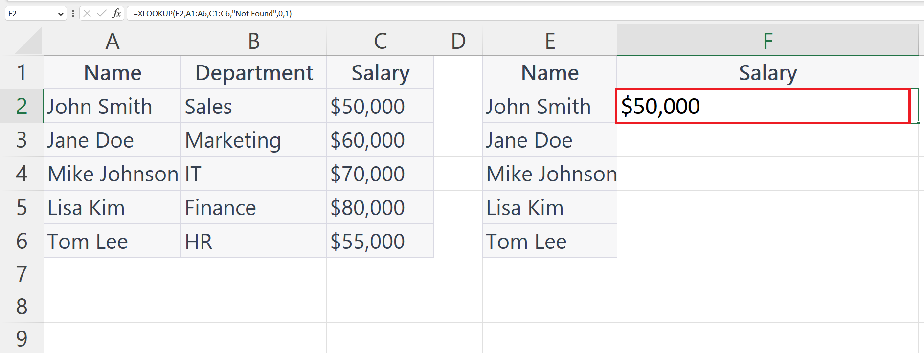
Here we have a dataset above showing Department and Salary of some employees. We will extract the salary of one of the employees i.e.John Smith from the data using the XLOOKUP function.
XLOOKUP is a powerful lookup function in Excel that allows you to search for a value in a range or an array and return a corresponding value from the same position in a different range or array. The XLOOKUP function is a versatile tool for data analysis and can save you time and effort when working with large datasets in Excel.
Step 1 – Select a Blank Cell
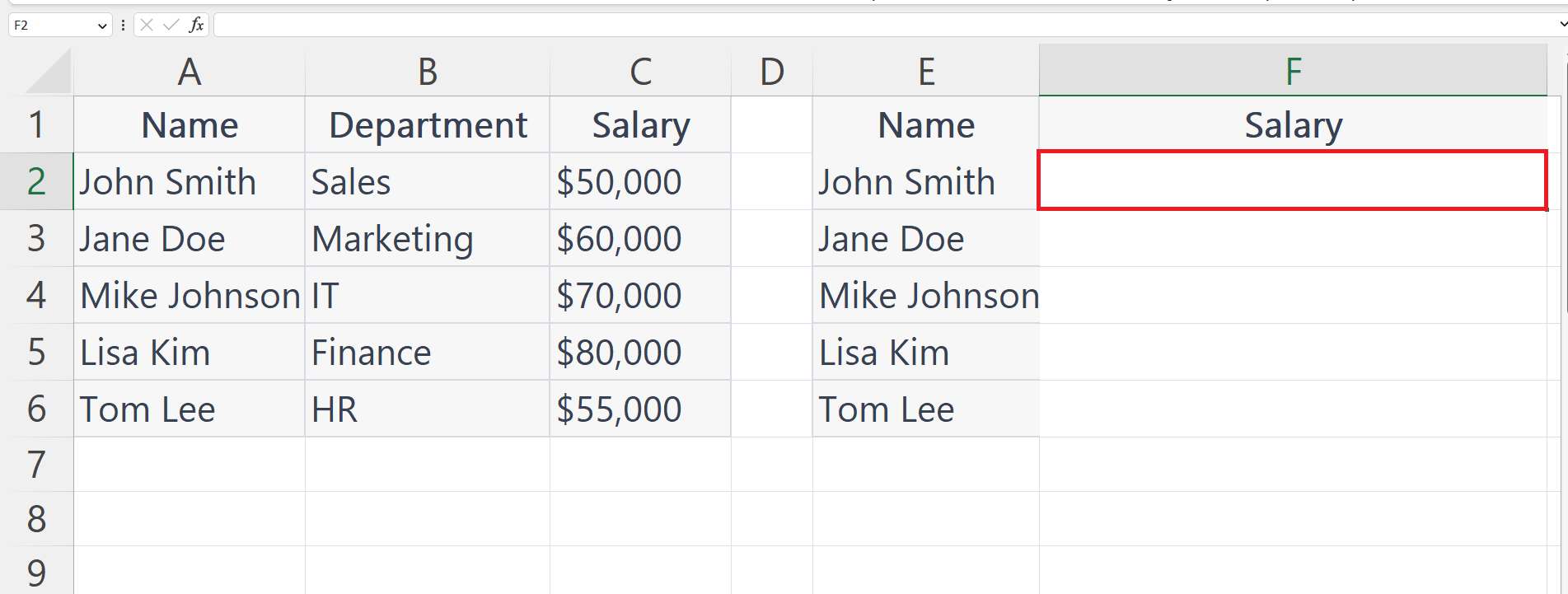
– Select a blank cell in which you want to extract the data.
Step 2 – Place an Equals Sign
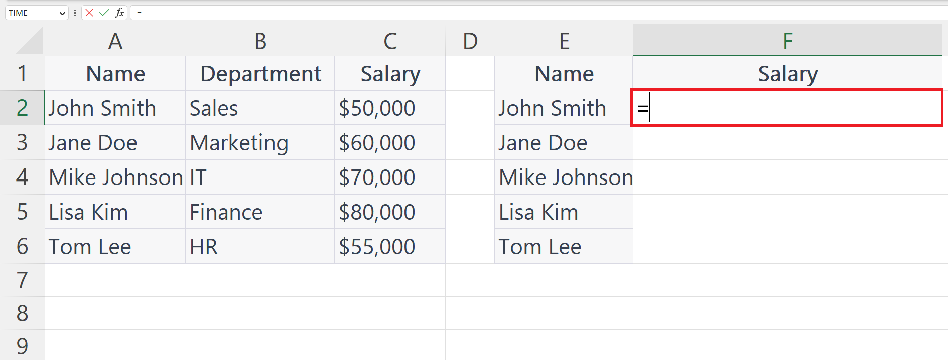
– Place an Equals Sign in the targeted blank cell.
Step 3 – Use the XLOOKUP Function
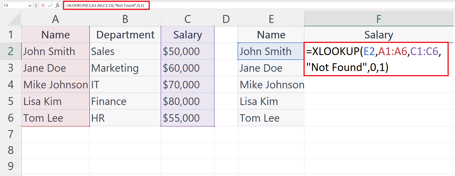
– Use the XLOOKUP function to extract the data from the data range.
Step 4 – Press the Enter Key
– Press the Enter key to extract the data.
Step 5 – Use Autofill to Extract Data for Each Employee

– Use the Autofill feature to extract data for each employee.


