
How do I sum colored cells in Excel
 By
SpreadCheaters
By
SpreadCheaters
You can watch a video tutorial here.
Using conditional formatting, it is possible to highlight cells based on their value. You can also choose to highlight cells by changing the background color of the cell. If you then need the sum of the colored cells, you can do so using the combination of a filter and a function.
Step 1 – Create the SUBTOTAL() function
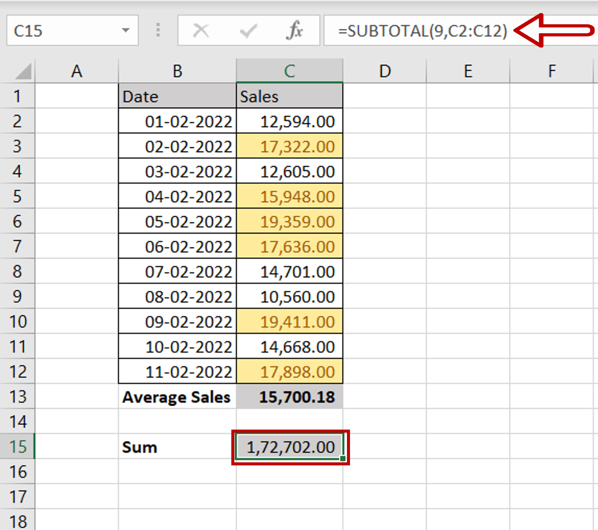
– In a cell below the table enter the formula using cell references:
=SUBTOTAL(9, <range of the ‘Sales’ column>)
Note: 9 represents the SUM function. When typing the SUBTOTAL() function, you will be prompted with a list of functions that can be used with SUBTOTAL()
Step 2 – Turn on the in-column filters
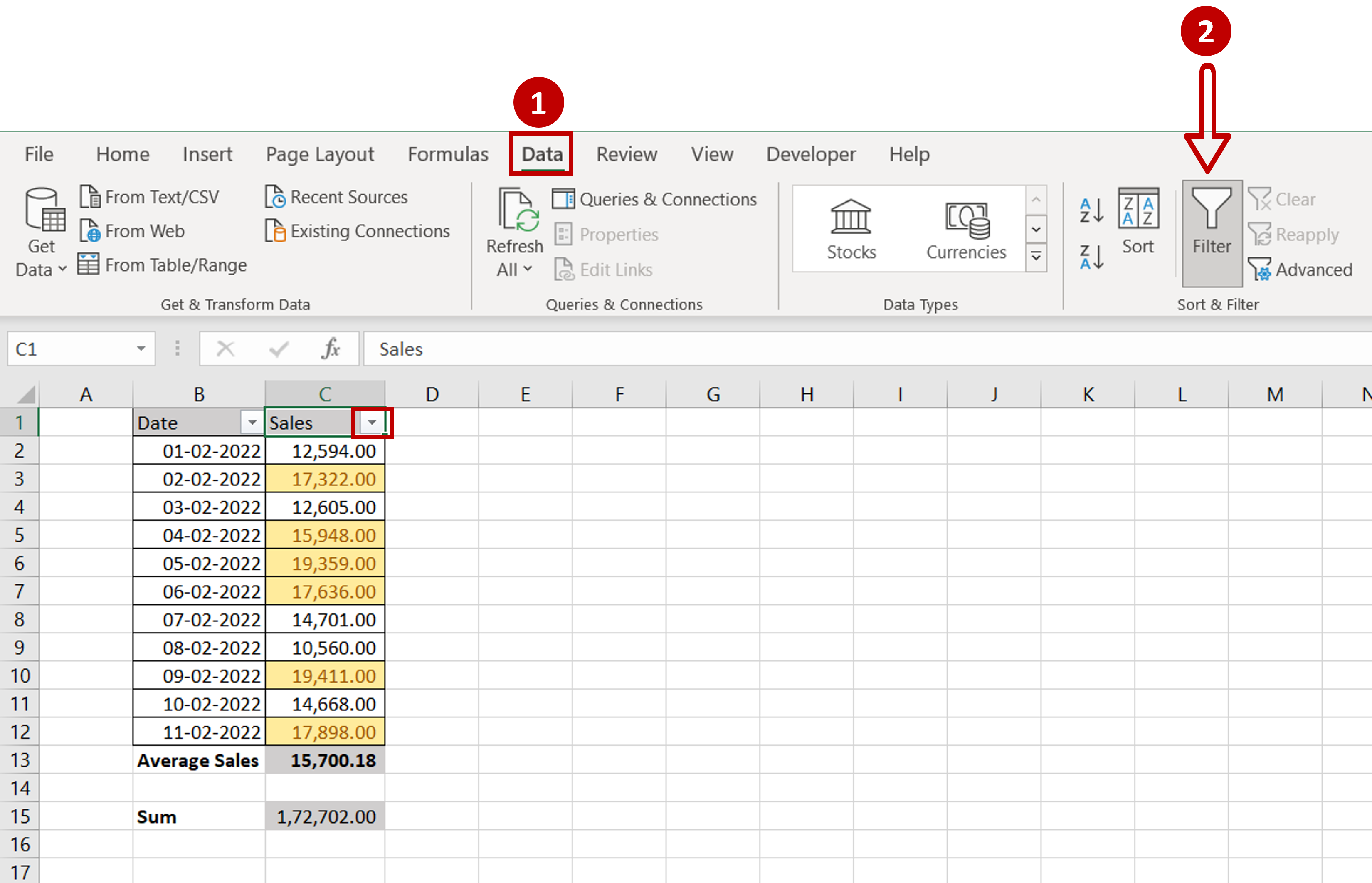
– Go to Data > Sort & Filter
– Click the Filter button
Step 3 – Choose the filter
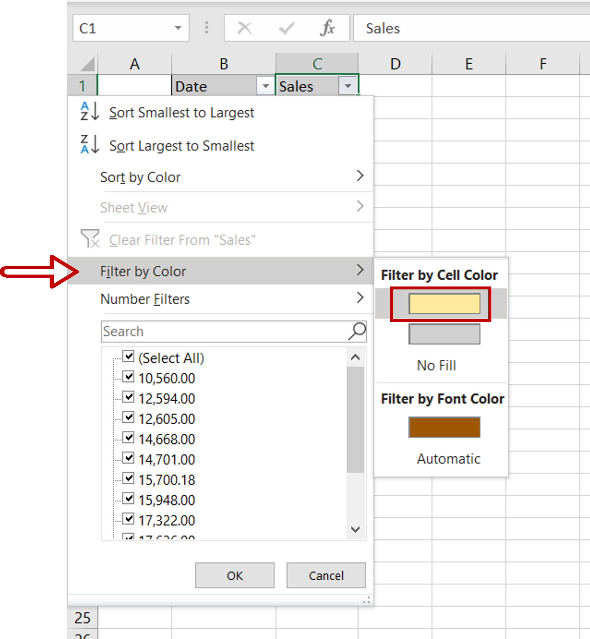
– On the filter drop-down menu, choose Filter by Cell Color
– Choose the color of the highlighted cells
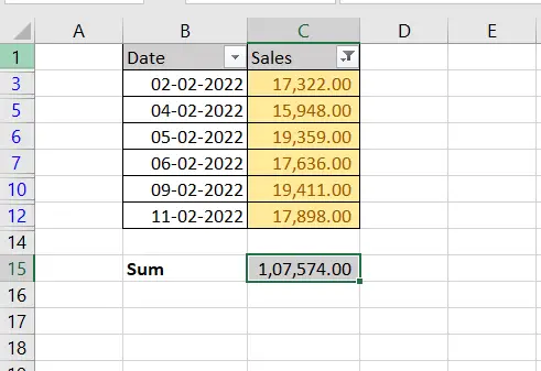
Step 4 – Check the sum
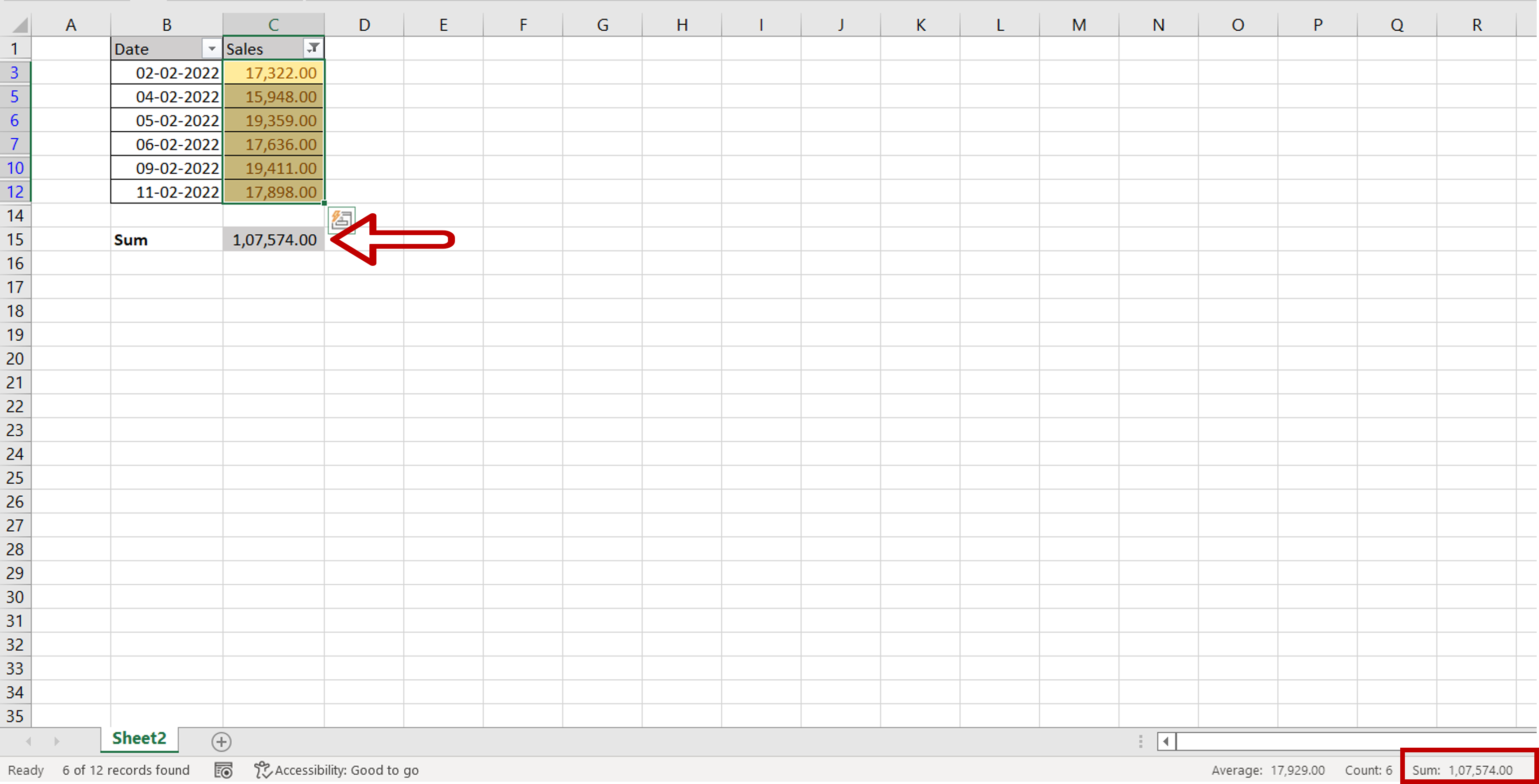
– Select the filtered cells
– On the bottom right of the sheet, the sum of the filtered cells is displayed
– The number will match that of the SUBTOTAL() function


